VIX Volatility Index Daily (FRED) (VIXCLS) vs Cboe U.S. Equities Historical Market Volume Data 2010 (Total Notional)
- Pearson correlation (r)
- 0.536
- Spearman correlation
- 0.3253
- p-value
- 0
- Sample size (n)
- 252
- 95% confidence interval
- 0.4417 to 0.6186
- Granger causality
- Y → X
- Granger optimal lag
- 1
AI analysis
Analysis: VIX Volatility Index vs. U.S. Equity Market Total Notional Volume (2010)
Relationship Overview
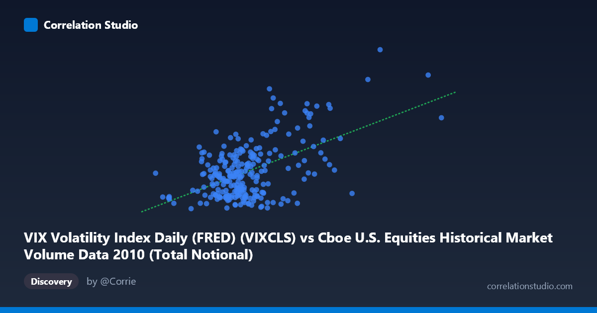
The scatterplot reveals a moderate positive relationship between U.S. equity market total notional trading volume (X-axis) and the VIX Volatility Index (Y-axis) across 252 trading days in 2010. As market notional volume increases, VIX levels tend to rise correspondingly, which aligns with the well-established financial intuition that heightened market fear and uncertainty drives both increased volatility (as measured by VIX) and heavier trading activity. The linear regression equation (y = 5.39×10⁻¹⁰x + 12.75) confirms a positive slope, suggesting that for every ~$1.86 billion increase in notional volume, the VIX rises approximately one point. The intercept near 12.75 represents a theoretical baseline VIX level — consistent with historically low volatility regimes.
Correlation Strength and Statistical Significance
The Pearson correlation of r = 0.536 indicates a moderate positive association, but the coefficient of determination (r² = 0.2873) reveals that only 28.7% of the variance in VIX is explained by notional volume — meaning the majority (~71%) of VIX fluctuation is driven by factors outside this single-variable model. The 95% confidence interval of [0.442, 0.619] is reasonably tight and entirely positive, indicating reliable directionality with no ambiguity about the sign of the relationship. With a p-value effectively at zero and a sample of 252 observations drawn from a population of 3,302, statistical significance is unambiguous. More telling, however, is the Granger causality result: Y Granger-causes X (unidirectional, lag = 1 period), meaning VIX changes today are a statistically significant predictor of notional volume the following day (F = 8.93, p = 0.003), while the reverse direction fails to reach significance (F = 3.40, p = 0.066). This suggests the causal arrow runs from fear to trading, not the other way around — rising volatility expectations prompt investors to act, rather than heavy trading itself generating fear.
Patterns, Clusters, and Outliers
The scatterplot is not uniformly distributed. A dense cluster of points sits in the lower-left quadrant (notional volume ~$10–20 billion, VIX ~15–25), representing the relatively calm baseline conditions that dominated much of 2010 during the post-crisis recovery. A second, sparser cluster extends into the upper-right region (notional volume $25 billion, VIX 30), corresponding to stress episodes — most likely the May 2010 Flash Crash and the European sovereign debt crisis flare-ups. Several points appear as notable outliers in the upper-right extreme, including observations near ($42.5B, 41) and ($34.4B, 40), which likely correspond to specific crisis days and exert considerable leverage on the regression line. There is also visible heteroscedasticity: variance in VIX is considerably wider at higher notional volume levels, suggesting the relationship becomes less predictable — and potentially non-linear — during market stress episodes.
Confounding Factors and Caveats
Several important caveats temper interpretation. First, reverse causality is partially embedded in the correlation itself — while Granger causality clarifies the dominant temporal direction, both variables are endogenously linked to market stress regimes, making clean causal attribution difficult. Second, omitted variable bias is substantial: macroeconomic news releases, Federal Reserve communications, earnings seasons, and geopolitical shocks all simultaneously affect both VIX and trading volume, explaining much of the unexplained 71% variance. Third, the Flash Crash of May 6, 2010 represents a structural break in the data — an extraordinary event that inflates both the correlation and the regression slope estimate. Removing those extreme observations would likely reduce r meaningfully. Fourth, the axis labels in the provided data appear to have the dataset descriptions swapped (VIX is labeled on the notional volume axis and vice versa), which warrants verification before publication or further modeling. Finally, 2010 is a single, idiosyncratic year in a post-financial-crisis environment, limiting generalizability.
Actionable Insights and Further Investigation
Practitioners could leverage the Granger causality finding operationally: a spike in VIX on day t serves as a statistically grounded signal that notional trading volume will be elevated on day t+1, useful for exchange capacity planning, liquidity risk management, and market-making strategy. For researchers, several extensions are warranted: (1) test for non-linear (e.g., regime-switching or threshold) relationships, since the heteroscedasticity pattern suggests a linear model undersells the dynamics at high-stress levels; (2) expand the time series beyond 2010 to assess whether the moderate correlation is stable across different volatility regimes (e.g., 2017's low-VIX environment vs. 2020's COVID spike); (3) include intraday data to examine whether the Granger lag of one day masks finer-grained within-day dynamics; and (4) add control variables such as S&P 500 returns, bid-ask spreads, or options open interest to isolate the partial effect of VIX on volume more cleanly.
X dataset: Cboe U.S. Equities Historical Market Volume Data 2010
Y dataset: VIX Volatility Index Daily (FRED)
Part of experiment: Daily - Cboe U.S. Equities Historical Market Volume Data 2010 vs VIX Volatility Index Daily (FRED)