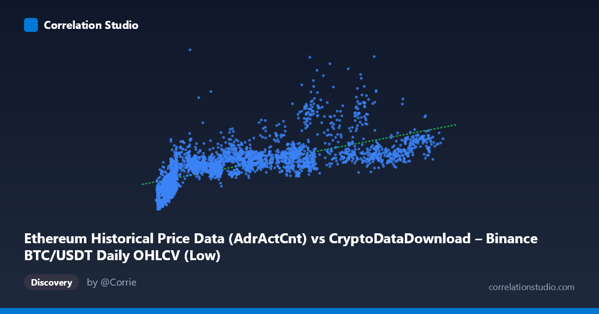
Ethereum Historical Price Data (AdrActCnt) vs CryptoDataDownload – Binance BTC/USDT Daily OHLCV (Low)
- Pearson correlation (r)
- 0.6933
- Spearman correlation
- 0.8272
- p-value
- 0
- Sample size (n)
- 3191
- 95% confidence interval
- 0.6748 to 0.7109
- Granger causality
- None
- Granger optimal lag
- 10
AI analysis
Analysis of the Relationship Between Ethereum Active Address Count and BTC/USDT Price
1. Overview of the Relationship
The scatterplot reveals a moderate positive association between the X variable (labeled as Ethereum Active Address Count, though the axis title suggests possible field mislabeling given the dataset descriptions) and the Y variable (BTC/USDT daily low price). As X increases from roughly 2,800 to 123,000, Y trends upward from the ~130K–150K range toward values exceeding 900K–1.5M. However, the scatter around the fitted line is substantial, particularly at low X values where Y ranges widely (from ~140K to ~770K when X is under 10,000), indicating that X alone is a weak-to-moderate predictor of Y in the lower range and a somewhat better predictor as X grows larger.
2. Strength, Direction, and Statistical Confidence
The Pearson correlation of r = 0.693 indicates a moderate-to-strong positive linear relationship, but r² = 0.481 means only about 48% of the variance in Y is explained by X — leaving over half of Y's variability attributable to other factors or noise. The 95% CI [0.675, 0.711] is tight given the large sample size (n=3,191), and the p-value of ~0 confirms this correlation is highly statistically significant and not due to chance. However, statistical significance here reflects sample size more than practical predictive strength — r² of 0.48 is a moderate fit, not a tight deterministic relationship. Critically, the Granger causality tests show no significant predictive direction in either direction (X→Y: p=0.686; Y→X: p=0.637). This is an important caveat: despite the contemporaneous correlation, neither variable appears to systematically lead or forecast the other in a time-series sense. This suggests the correlation may reflect a shared external driver (e.g., both being influenced by overall crypto market cycles or macro liquidity conditions) rather than one variable causing changes in the other.
3. Patterns, Clusters, and Non-linearity
Several notable features emerge from the sample data: - Heteroscedasticity: The spread of Y increases as X increases — at low X (~4,000–10,000), Y values cluster more tightly in the 140K–500K range, but at higher X (~60,000–110,000), Y values spread more widely (540K to 1,500K+). - Possible curvature: The note that Spearman ρ exceeds Pearson r is a strong signal of non-linearity — likely a logarithmic or power-law relationship rather than a straight line, which is common in crypto data where growth is often exponential or log-distributed. - Outlier cluster: Points like (65712, 999185) and (63888, 976428) and (89314, 860816) sit well above the regression line, suggesting a possible secondary regime or bull-market period where Y rises disproportionately relative to X. - Low-X plateau: Multiple points near X≈4,000–10,000 show Y values from 140K to over 500K, indicating that at low activity levels, price is driven by other factors (likely broader market sentiment/cycle stage rather than address activity).
4. Confounding Factors and Caveats
Several caveats limit causal interpretation: - Field/label mismatch: The stated axis descriptions are inconsistent (X labeled as Ethereum AdrActCnt but sourced from a Binance BTC/USDT OHLCV dataset; Y labeled as BTC/USDT Low but sourced from an Ethereum metrics dataset). This suggests possible data pipeline mislabeling that should be verified before drawing strong conclusions. - Time trend confound: Both crypto prices and network activity metrics tend to trend upward over multi-year periods (2017–2026) due to overall market growth/adoption cycles. This shared temporal trend can inflate correlation without indicating direct interaction — classic spurious correlation risk in trending time series. - Non-stationarity: Price and address-count series are typically non-stationary (trending, volatile), which can bias both Pearson correlation and Granger causality results. Proper differencing or detrending is needed before causal inference. - Third-variable influence: Overall crypto market capitalization, Bitcoin halving cycles, or macro liquidity (interest rates, ETF flows) likely drive both variables simultaneously.
5. Actionable Insights and Next Steps
1. Verify data provenance: Resolve the labeling inconsistency between axis titles and dataset descriptions before further analysis — this is critical for correct interpretation. 2. Test non-linear models: Given Spearman Pearson, fit log-log or polynomial regressions; a log transformation of both variables (common for price/activity data) may substantially improve fit and better reflect the underlying multiplicative relationship. 3. De-trend and re-test causality: Since raw levels show no Granger causality, apply first-differencing or use returns/growth rates and re-run Granger tests — this often reveals hidden lead-lag relationships masked by shared trends in level data. 4. Segment by market regime: Given the heteroscedastic spread, consider splitting the data into bull/bear market periods or by time era to check if the correlation strength and slope differ across regimes. 5. Include control variables: Incorporate broader market indicators (total crypto market cap, BTC dominance, macro liquidity indices) in a multivariate model to isolate the direct relationship between these two series from common external drivers.
X dataset: CryptoDataDownload – Binance BTC/USDT Daily OHLCV
Y dataset: Ethereum Historical Price Data
Part of experiment: Bitcoin - CryptoDataDownload – Binance BTC/USDT Daily OHLCV vs Ethereum Historical Price Data