World Bank CO2 Emissions by Country (DataBank) (Gas Fuel) vs US Employment and Unemployment (nonagriculture_ratio)
- Pearson correlation (r)
- 0.9761
- Spearman correlation
- 0.9883
- p-value
- 0
- Sample size (n)
- 80
- 95% confidence interval
- 0.9629 to 0.9846
- Granger causality
- None
- Granger optimal lag
- 10
- Time coverage
- 1941-01-01 to 2020-01-01
AI analysis
Scatterplot Analysis: Gas Fuel CO2 Emissions vs. US Non-Agriculture Employment Ratio
1. Overall Relationship
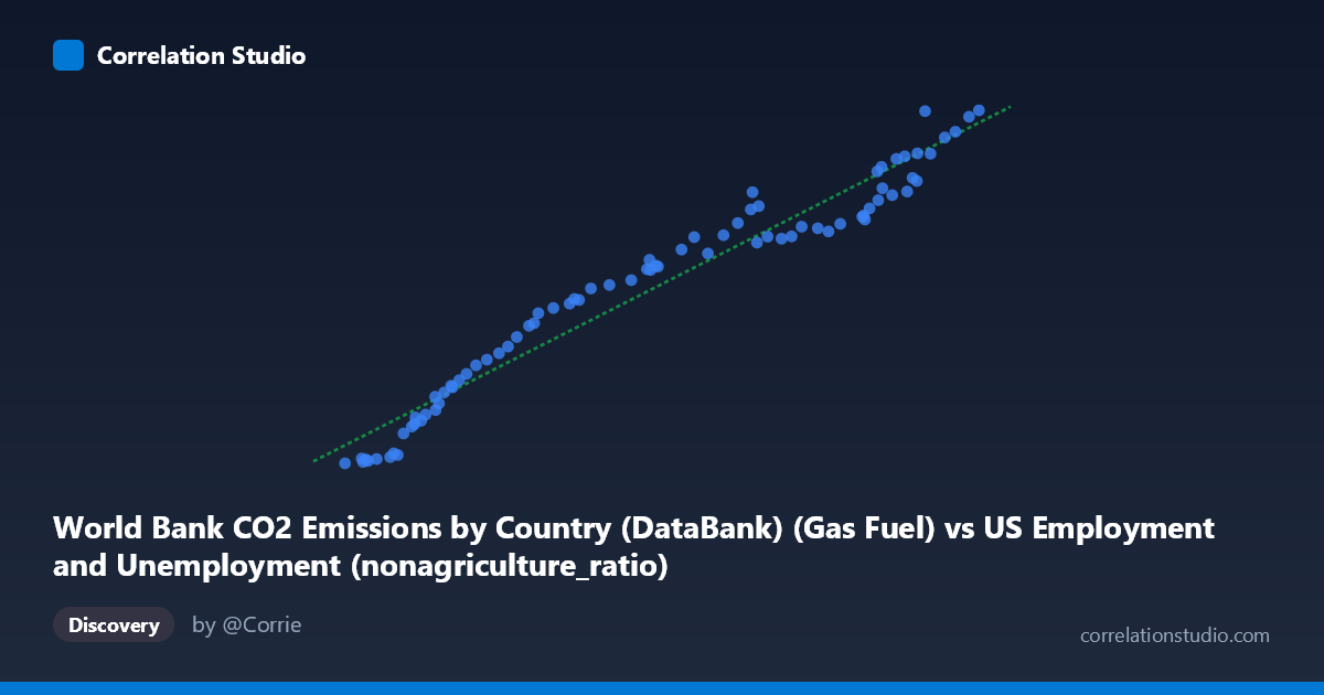
The scatterplot reveals a strikingly strong, positive, and approximately linear relationship between World Bank gas fuel CO2 emissions and the US non-agriculture employment ratio over the period 1941–2020. As gas fuel emissions increase across the X-axis range (~41,250 to ~155,113 units), the non-agriculture employment ratio rises correspondingly from roughly 654 to nearly 16,992. The data points cluster tightly around the regression line (y = 0.131085x − 3,916.07), suggesting that both variables have grown in a remarkably consistent, near-parallel trajectory across eight decades. This long-run co-movement is visually unmistakable and reflects the shared upward trend of industrialization, energy consumption, and structural labor market shifts that characterized the post-WWII era in the United States and globally.
2. Correlation Strength, Direction, and Causality
The correlation is exceptionally strong (r = 0.9761), and the R² of 0.9528 means that approximately 95.3% of the variance in the non-agriculture employment ratio is statistically explained by gas fuel CO2 emissions within this linear model — an unusually high figure for social and economic data spanning 80 years. The 95% confidence interval for r [0.9629, 0.9846] is narrow and sits entirely in the upper range of strong correlation, and the p-value of effectively 0 confirms this relationship is extremely unlikely to be a statistical artifact of sampling. However, the Granger causality tests critically undermine any causal narrative: neither direction (X→Y: F=1.04, p=0.43; Y→X: F=0.77, p=0.65) achieves statistical significance, even at an optimal lag of 10 periods. This means that knowing past values of gas emissions does not significantly improve predictions of future employment ratios, and vice versa. The high correlation reflects shared temporal trend, not predictive causation.
3. Notable Patterns, Clusters, and Outliers
The data distribute relatively smoothly along the regression line with no dramatic gaps, consistent with annual time-series data following a secular trend. However, there are a few notable features. At the lower end of the X-axis (roughly 41,250–65,000), the data points show somewhat greater scatter around the regression line, suggesting more variability in the early decades (1940s–1960s) when both the labor market structure and energy systems were still rapidly evolving. At the upper end (X 130,000), points again show mild dispersion — some sitting notably above the line (e.g., ~145,446 X with Y ~16,954) and others slightly below — possibly reflecting the post-2000 period when US employment ratios were influenced by recessions (2001, 2008–09) while emissions continued on a different trajectory. No single extreme outlier dramatically distorts the fit, but the point at (155,113; 16,992) anchors the upper extreme and warrants scrutiny as it may represent a specific peak year.
4. Confounding Factors and Caveats
The most critical caveat is that both variables are time-trending series, and high correlations between trending variables are a well-known statistical hazard — they frequently reflect nothing more than shared long-run growth, a phenomenon called spurious correlation. The Granger test's failure to find directional predictive power strongly supports this interpretation. Additional confounders abound: US GDP growth, population expansion, post-war industrialization, and global energy demand have driven both gas CO2 emissions and non-agricultural employment simultaneously, without one causing the other. The dataset labels also raise a flag — the X-axis column is drawn from a "US Employment" dataset while labeled as CO2 emissions, and the Y-axis originates from a CO2 dataset but measures employment ratio, suggesting possible dataset join or labeling complexity that should be verified. Finally, the non-agriculture employment ratio is influenced by demographic shifts, automation, and service-sector growth that have little mechanistic connection to fossil fuel combustion.
5. Actionable Insights and Further Investigation
Given the spurious trend correlation risk, the most important next step is to detrend both series (e.g., using first-differences or HP filtering) and re-examine the correlation on residuals — if the strong r collapses toward zero, the relationship is confirmed as trend-driven rather than structurally meaningful. Researchers should also test for cointegration (e.g., Engle-Granger or Johansen tests), which would determine whether the variables share a statistically meaningful long-run equilibrium beyond common trending. It would be valuable to extend Granger causality testing with shorter lag windows and across sub-periods (pre/post-1980) to detect any era-specific predictive relationships masked by the full-period aggregate. Finally, introducing control variables — GDP, population, energy mix transitions, and major economic shocks — into a multivariate framework would help isolate whether any residual relationship between gas emissions and labor structure persists once shared macro drivers are accounted for.
X dataset: US Employment and Unemployment
Y dataset: World Bank CO2 Emissions by Country (DataBank)
Part of experiment: Yearly - US Employment and Unemployment vs World Bank CO2 Emissions by Country (DataBank)