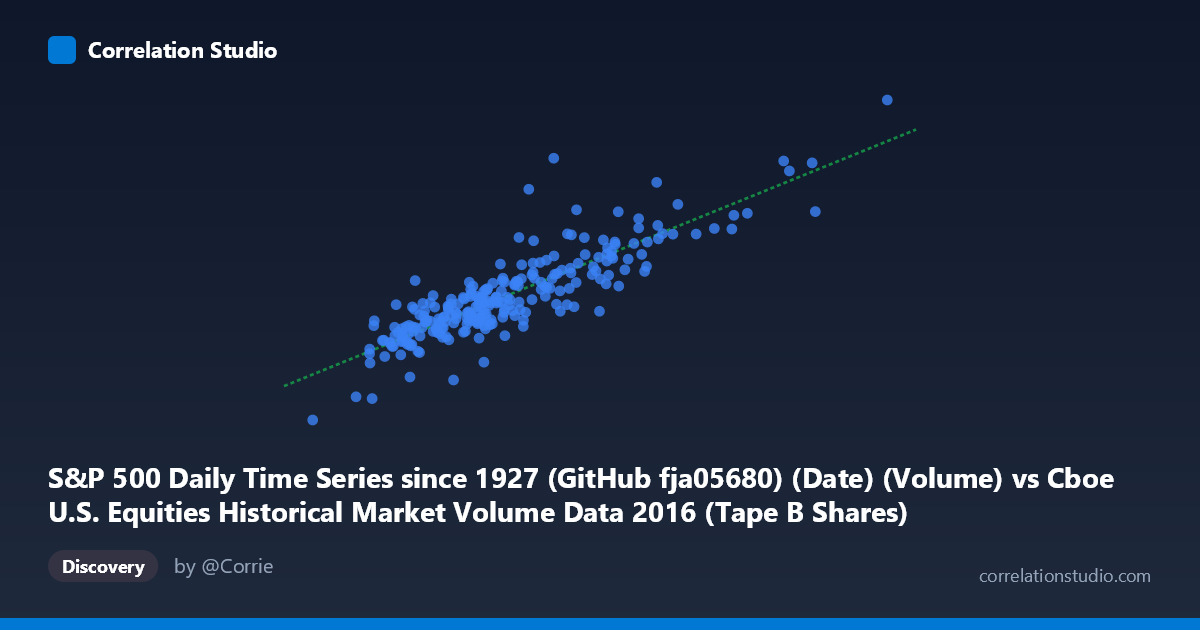
S&P 500 Daily Time Series since 1927 (GitHub fja05680) (Date) (Volume) vs Cboe U.S. Equities Historical Market Volume Data 2016 (Tape B Shares)
- Pearson correlation (r)
- 0.8665
- Spearman correlation
- 0.8536
- p-value
- 0
- Sample size (n)
- 252
- 95% confidence interval
- 0.832 to 0.8943
- Granger causality
- None
- Granger optimal lag
- 10
AI analysis
Analysis: S&P 500 Daily Volume vs. Cboe Tape B Shares (2016)
Relationship Overview The scatterplot reveals a clear positive linear relationship between S&P 500 daily trading volume and Cboe Tape B shares traded across 252 trading days in 2016. As overall market volume increases, Tape B share activity rises proportionally, which is broadly intuitive — Tape B covers NYSE American (AMEX)-listed securities, and its activity tends to move in concert with broader U.S. equity market participation. The linear regression equation (y = 23.027x + 1.438B) suggests that for every additional unit of S&P 500 volume, Tape B shares increase by approximately 23 units, with a substantial baseline intercept reflecting persistent Tape B activity independent of S&P 500 volume fluctuations.
Correlation Strength and Statistical Significance The correlation is strong and positive (r = 0.867), and critically, r² = 0.751 indicates that approximately 75.1% of the variance in Tape B shares is explained by S&P 500 volume — a substantively meaningful proportion. The 95% confidence interval [0.832, 0.894] is narrow and excludes zero by a wide margin, and the p-value of effectively zero confirms this relationship is not a chance artifact in a sample of n = 252 from a population of N = 3,622. However, the Granger causality results tell a more nuanced story: neither direction of temporal prediction is statistically significant (X→Y: F = 0.575, p = 0.833; Y→X: F = 0.504, p = 0.886), even at an optimal lag of 10 periods. This means that while the two series move together strongly in a contemporaneous sense, knowing yesterday's S&P 500 volume does not help predict today's Tape B shares any better than baseline, and vice versa. The relationship is correlational and likely driven by shared contemporaneous factors rather than any directional lead-lag dynamic.
Patterns, Clusters, and Outliers The data cloud is relatively well-behaved along the regression line for the bulk of observations clustered between roughly 70M–130M on the X-axis and 3B–4.5B on the Y-axis. However, several notable features stand out. There are high-leverage outliers in the upper-right region — points exceeding 150M–170M in S&P 500 volume with Tape B shares approaching or exceeding 5B — which likely correspond to days of elevated market stress or major macro events (e.g., Brexit aftermath in June 2016, U.S. election day in November). A smaller cluster appears at the lower-left extreme, representing unusually quiet sessions. The spread of residuals appears to widen slightly at higher volume levels, hinting at mild heteroscedasticity, which is common in financial volume data and slightly undermines the assumption of uniform variance in OLS regression.
Confounds and Caveats Several important caveats apply. First, both variables are fundamentally market volume measures — they share structural drivers such as macroeconomic announcements, earnings seasons, index rebalancing, and volatility regimes. This common driver inflation makes the high r² less surprising and potentially less informative than it first appears. Second, the axis labeling warrants scrutiny: the dataset notes suggest the Y-axis ("Tape B Shares") is drawn from the S&P 500 dataset and the X-axis volume from the Cboe dataset, which may reflect a metadata crosswalk issue — analysts should verify column-to-dataset alignment before drawing firm conclusions. Third, 2016 is a single calendar year with idiosyncratic events (Brexit, U.S. elections), limiting generalizability across other market regimes. Finally, the absence of Granger causality at up to 10 lags suggests no exploitable temporal structure, but longer lags or nonlinear causality frameworks (e.g., transfer entropy) were not tested.
Actionable Insights and Further Investigation Despite the strong contemporaneous correlation, the lack of Granger causality means this relationship should not be used for short-term prediction in isolation. Practitioners could investigate whether the relationship holds across multiple years and market regimes, or whether it breaks down during periods of structural market change (e.g., COVID-era volume surges). It would be valuable to decompose residuals to identify which specific dates the model misfits most severely — these outlier days likely carry interpretable market narratives. Analysts should also test whether volatility (VIX) or macroeconomic surprise indices serve as the latent common driver, which could sharpen causal inference. Finally, extending the analysis to other Tape classifications (A, C) would clarify whether Tape B's relationship to total S&P 500 volume is structurally distinct or simply mirrors aggregate market behavior.
X dataset: Cboe U.S. Equities Historical Market Volume Data 2016
Y dataset: S&P 500 Daily Time Series since 1927 (GitHub fja05680) (Date)
Part of experiment: Daily - Cboe U.S. Equities Historical Market Volume Data 2016 vs S&P 500 Daily Time Series since 1927 (GitHub fja05680) (Date)