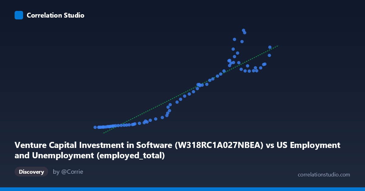
Venture Capital Investment in Software (W318RC1A027NBEA) vs US Employment and Unemployment (employed_total)
- Pearson correlation (r)
- 0.9447
- Spearman correlation
- 0.9595
- p-value
- 0
- Sample size (n)
- 79
- 95% confidence interval
- 0.9147 to 0.9644
- Granger causality
- None
- Granger optimal lag
- 10
- Time coverage
- 1946-01-01 to 2024-01-01
AI analysis
Scatterplot Analysis: Venture Capital Software Investment vs. Total US Employment
1. Overall Relationship
The scatterplot reveals a strong, positive relationship between Venture Capital Investment in Software (X) and Total US Employment (Y) across the 1946–2024 period. As software investment grows, total employment rises correspondingly, tracing a broadly upward trajectory. The linear regression equation (y = 0.00396x − 265.938) captures this trend well at a macro level, though the scatter becomes noticeably wider at higher investment values, hinting at increasing variability as the economy scales. The data span nearly eight decades, meaning this chart effectively compresses long-run structural changes in the US economy into a single cross-sectional view.
2. Correlation Strength, Direction, and Temporal Predictive Power
The Pearson correlation of r = 0.9447 indicates a very strong positive association, and the R² = 0.8925 means approximately 89.2% of the variance in total employment is statistically explained by software investment levels — a remarkably high figure for macroeconomic data of this complexity. The 95% confidence interval [0.9147, 0.9644] is narrow and sits entirely in strongly positive territory, confirming this is not a sampling artifact, and the p-value of ~0 renders the result highly statistically significant. However, the Granger causality results critically temper any causal interpretation: neither direction shows significant predictive power (X→Y: F = 0.39, p = 0.95; Y→X: F = 0.57, p = 0.83). Even at the optimal lag of 10 periods, neither variable reliably predicts the other temporally. This means the correlation, however strong, reflects co-movement rather than directional causation — both series are likely being driven by shared underlying forces rather than one causing the other.
3. Patterns, Clusters, and Outliers
The data naturally cluster into two distinct regimes visible in the scatterplot. A dense lower-left cluster exists where X < ~90,000 and Y < ~50 — corresponding to the pre-digital era (roughly pre-1990s) when software investment was minimal and employment was lower. A second, more dispersed upper-right cloud spans higher investment and employment values, reflecting the post-1990s tech boom era. Several points warrant attention as potential outliers: the observation at (146,047; 455.02) and (145,362; 466.42) sit noticeably above the regression line at high X values, suggesting periods where employment surged beyond what investment alone would predict. Conversely, some high-X, moderate-Y points (e.g., ~153,000–158,000 range yielding Y ~270–304) fall below the trend line, indicating episodes where large software investment did not translate proportionally into employment gains — possibly reflecting automation, efficiency gains, or post-bubble corrections.
4. Confounding Factors and Caveats
The most significant caveat is the classic spurious correlation risk with long-run time series: both software investment and total employment grow over time due to population growth, GDP expansion, inflation, and broader technological development. Any two upward-trending series over 78 years will tend to correlate strongly without there being a meaningful direct relationship. The absence of Granger causality reinforces this concern. Additionally, the dataset label descriptions appear to have their axes swapped in the metadata (X is labeled from an employment dataset, Y from a VC/software dataset), which may indicate a data pipeline inconsistency worth verifying. Omitted variables — including interest rates, government spending, immigration trends, and global trade cycles — almost certainly explain substantial portions of both series' movements. The wide scatter at high X values also suggests heteroscedasticity, which violates linear regression assumptions and may inflate R².
5. Actionable Insights and Further Investigation
Given the strong co-movement but absent Granger causality, analysts should avoid policy claims that increasing software investment will directly grow employment or vice versa. Instead, this relationship is better treated as a macro indicator of shared economic expansion phases. Recommended next steps include: (a) controlling for GDP or population to test whether the partial correlation survives; (b) decomposing the time series to remove shared trends before re-running Granger tests; (c) segmenting analysis pre- and post-1990 to test whether the relationship differs across economic eras; (d) investigating the outlier years (especially the high-employment, high-investment points) to understand what sector-specific or policy factors drove deviations; and (e) verifying the dataset column-to-axis mapping to confirm no labeling errors before publishing conclusions.
X dataset: US Employment and Unemployment
Y dataset: Venture Capital Investment in Software
Part of experiment: Yearly - US Employment and Unemployment vs Venture Capital Investment in Software