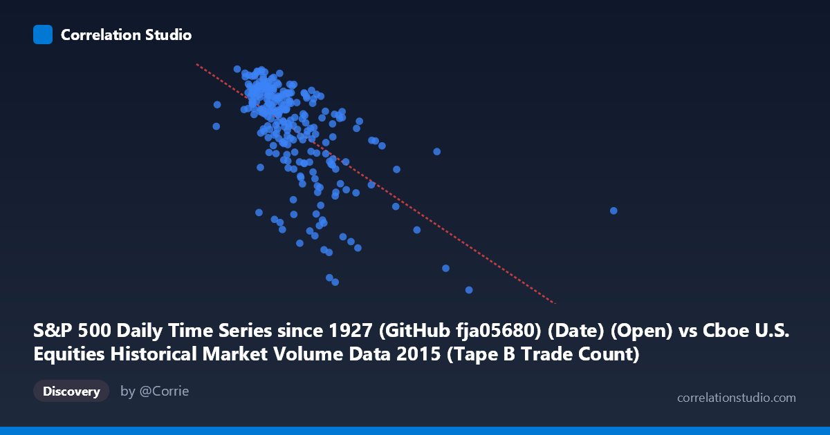
S&P 500 Daily Time Series since 1927 (GitHub fja05680) (Date) (Open) vs Cboe U.S. Equities Historical Market Volume Data 2015 (Tape B Trade Count)
- Pearson correlation (r)
- -0.5996
- Spearman correlation
- -0.6614
- p-value
- 0
- Sample size (n)
- 252
- 95% confidence interval
- -0.6733 to -0.5141
- Granger causality
- None
- Granger optimal lag
- 1
AI analysis
Analysis: S&P 500 Opening Price vs. Cboe Tape B Trade Count (2015)
Relationship Overview The scatterplot reveals a moderate negative relationship between the S&P 500 daily opening price (X) and the Cboe Tape B trade count (Y) across 2015 trading days. As the S&P 500 opening price increases, the number of Tape B trades tends to decrease. The linear regression equation (y = −0.000351x + 2,166.25) quantifies this inverse slope, suggesting that for every 100,000-point increase in the opening price index value, Tape B trade counts decline by roughly 35 units. Visually, the bulk of observations cluster in the lower X range (roughly 130,000–400,000) with Y values concentrated between ~1,900 and 2,130, while a sparse tail of high-X outliers stretches rightward with notably lower Y values.
Correlation Strength, Direction, and Causality The Pearson correlation of r = −0.5996 indicates a moderate-to-strong negative association, statistically significant with a p-value effectively at zero. The 95% confidence interval [−0.6733, −0.5141] is reassuringly narrow, confirming this is not a sampling artifact. However, the R² of 0.3595 is the more sobering figure — the S&P 500 opening price explains only ~36% of the variance in Tape B trade counts, meaning roughly 64% of the variation remains unexplained by this single predictor. Critically, the Granger causality tests find no significant temporal predictive direction in either direction (X→Y: p = 0.9987; Y→X: p = 0.7669), meaning that knowing today's S&P 500 opening price does not meaningfully help predict tomorrow's Tape B trade count, and vice versa. The correlation reflects co-movement, not a predictive or causal mechanism.
Notable Patterns, Clusters, and Outliers The data exhibits a clear dense core cluster between X values of ~175,000–375,000 and Y values of ~1,900–2,130, representing the vast majority of typical 2015 trading days. Beyond X ≈ 400,000, observations become sparse and consistently show depressed Y values (below ~2,050), suggesting high-price-level days are associated with lower Tape B activity. Several points in this high-X tail — including observations near (621,009, 2,034) and (640,679, 1,898) — appear as potential outliers that may be disproportionately influencing the regression slope. There is also a visible lower band of points with Y values around 1,872–1,950 scattered at mid-to-high X values, hinting at possible regime-distinct trading sessions (e.g., low-volume holiday-adjacent days or market stress periods).
Confounding Factors and Caveats The most important caveat here is the dataset join structure: X comes from S&P 500 price history while Y comes from Cboe market volume data, merged on date. The apparent inverse relationship likely reflects a shared temporal confound — during 2015, the S&P 500 experienced a notable summer correction (August 2015), and market volatility events tend to simultaneously elevate volume/trade counts while depressing price levels. This means the correlation may largely capture time-driven co-variation rather than any structural link between price levels and Tape B activity. Additionally, Tape B covers NYSE American and regional exchange securities specifically, so its trade count dynamics may be only loosely coupled to broad S&P 500 index movements. The high-X outliers likely correspond to specific notional value scaling differences rather than genuine price-level extremes.
Actionable Insights and Further Investigation Given the moderate but unexplained variance and absent Granger causality, practitioners should not use S&P 500 opening price as a standalone predictor of Tape B trade counts. A more productive path would be to (1) incorporate VIX or realized volatility as a covariate, which likely explains much of the residual 64% variance; (2) disaggregate by market regime (pre/post August 2015 correction) to test whether the correlation is stable or driven by a single volatility episode; (3) examine the high-X outliers more closely to determine if they represent data anomalies or genuine structural sessions; and (4) test longer lags (2–5 periods) in Granger causality, as the current analysis only evaluated lag-1. Understanding whether this correlation persists in other years would also help distinguish genuine structural coupling from a 2015-specific artifact.
X dataset: Cboe U.S. Equities Historical Market Volume Data 2015
Y dataset: S&P 500 Daily Time Series since 1927 (GitHub fja05680) (Date)
Part of experiment: Daily - Cboe U.S. Equities Historical Market Volume Data 2015 vs S&P 500 Daily Time Series since 1927 (GitHub fja05680) (Date)