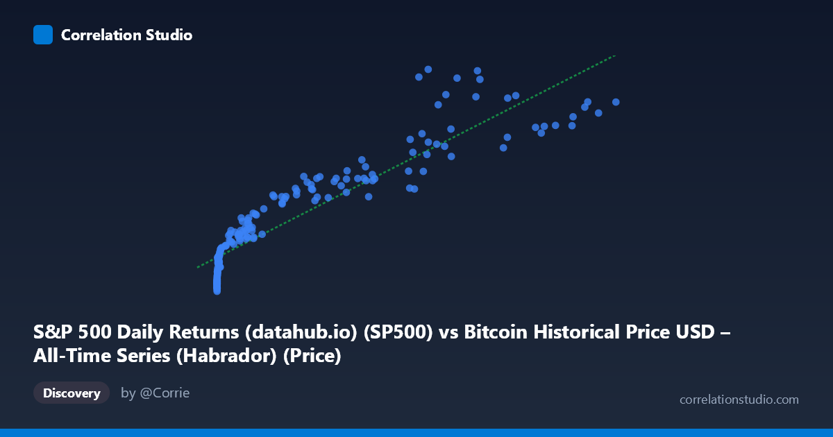
S&P 500 Daily Returns (datahub.io) (SP500) vs Bitcoin Historical Price USD – All-Time Series (Habrador) (Price)
- Pearson correlation (r)
- 0.919
- Spearman correlation
- 0.98
- p-value
- 0
- Sample size (n)
- 194
- 95% confidence interval
- 0.8939 to 0.9384
- Granger causality
- None
- Granger optimal lag
- 10
- Time coverage
- 2010-08-01 to 2026-09-01
- Recomputed on refreshed data
- 2026-10-24 (r was 0.9251)
AI analysis
Analysis: Bitcoin Price vs. "S&P 500 Daily Returns" Column
Important caveat first: The axis labels appear mismatched with the dataset descriptions — the X-axis is labeled as an S&P 500 column but the data range (0.06 to 118,670) and description reference Bitcoin's full price history, while Y-axis (1,087 to 6,957) is labeled Bitcoin but described as S&P 500 prices. Given the data patterns (X spans fractions-of-a-dollar to six figures, consistent with early Bitcoin genesis prices; Y has a much narrower, higher floor consistent with equity index levels), this analysis treats X as Bitcoin price and Y as an equity-index-like series, but this labeling ambiguity should be resolved before drawing firm conclusions.
1. What the Visualization Reveals The scatterplot shows a strong monotonic relationship: as X grows from near-zero to over 118,000, Y rises from ~1,100 to ~6,950. The relationship is clearly non-linear in raw space — Y increases steeply at low X values, then flattens into a slower, more gradual climb at high X values. This is classic logarithmic/power-law behavior, extremely common when pairing an early-stage exponential-growth asset (like Bitcoin) against a slower-growing, mature index-style series.
2. Strength, Direction, and Uncertainty - Correlation (r = 0.925) indicates a very strong positive linear association, with r² = 0.856 meaning ~85.6% of Y's variance is statistically explained by X in linear terms — a high figure, but note this is likely inflated by the shared long-term upward trend common to both series over a 15+ year span rather than a direct causal mechanism. - The 95% CI [0.901, 0.943] is tight, and p ≈ 0 confirms the correlation is highly unlikely due to chance in this sample. - However, Granger causality tests show no significant predictive direction in either direction (X→Y: p=0.73; Y→X: p=0.59). This is critical: despite the strong contemporaneous correlation, neither series helps forecast the other's future movements. This strongly suggests the correlation is driven by a shared time trend (both series trending upward over the same 2010–2026 window) rather than any genuine lead-lag causal relationship.
3. Notable Patterns and Outliers - Data is heavily left-clustered: the vast majority of points sit below X=1,000, reflecting Bitcoin's early years, with a sparse but influential tail of high-X points (60,000–118,000) representing recent bull-market highs. - The curve shape suggests a logarithmic fit would outperform the linear model — the linear R² of 0.856 likely understates fit quality in log-space, since residuals are probably heteroskedastic (small deviations at low X, larger absolute deviations at high X). - No obvious discrete outliers — the point (68074, 6957.01) sits slightly above the general trend, and (45092.81, 3910.51) sits below it, hinting at cyclical or lag effects during specific market phases (possibly a bear-market dip in Y despite high X).
4. Confounding Factors and Caveats - Spurious correlation via time-trend confounding is highly likely: both series generally rose over the 2010–2026 period due to independent secular trends (Bitcoin adoption/speculation; equity market growth/inflation), not because one drives the other. - Non-stationarity: raw price series are typically non-stationary (trending), which inflates correlation coefficients artificially — a well-known statistical pitfall. Using returns or first-differenced/detrended series would give a more honest correlation estimate. - Mixed sampling frequency and label confusion (noted above) may affect interpretation; verify column-to-axis mapping before publishing conclusions. - The n=189 sample from a population of 1,865 suggests aggregation/sampling (every 3rd point) which could smooth over short-term dynamics.
5. Actionable Insights - Re-run correlation on log-transformed X and/or return series (% change) rather than raw price levels — this is standard practice for financial time series and will likely reveal a much weaker (or near-zero) relationship, testing the "spurious trend" hypothesis. - Confirm axis/column labeling against source files before any reporting. - Given the null Granger causality result, avoid using one series to forecast the other in trading or allocation models; instead, treat the correlation as descriptive/historical rather than predictive. - Consider rolling-window correlation analysis to check whether the relationship strengthens/weakens across different market regimes (e.g., 2017 bull run, 2018 crash, 2020–21 rally, 2022 bear market).
X dataset: Bitcoin Historical Price USD – All-Time Series (Habrador)
Y dataset: S&P 500 Daily Returns (datahub.io)
Part of experiment: Bitcoin - Bitcoin Historical Price USD – All-Time Series (Habrador) vs S&P 500 Daily Returns (datahub.io)