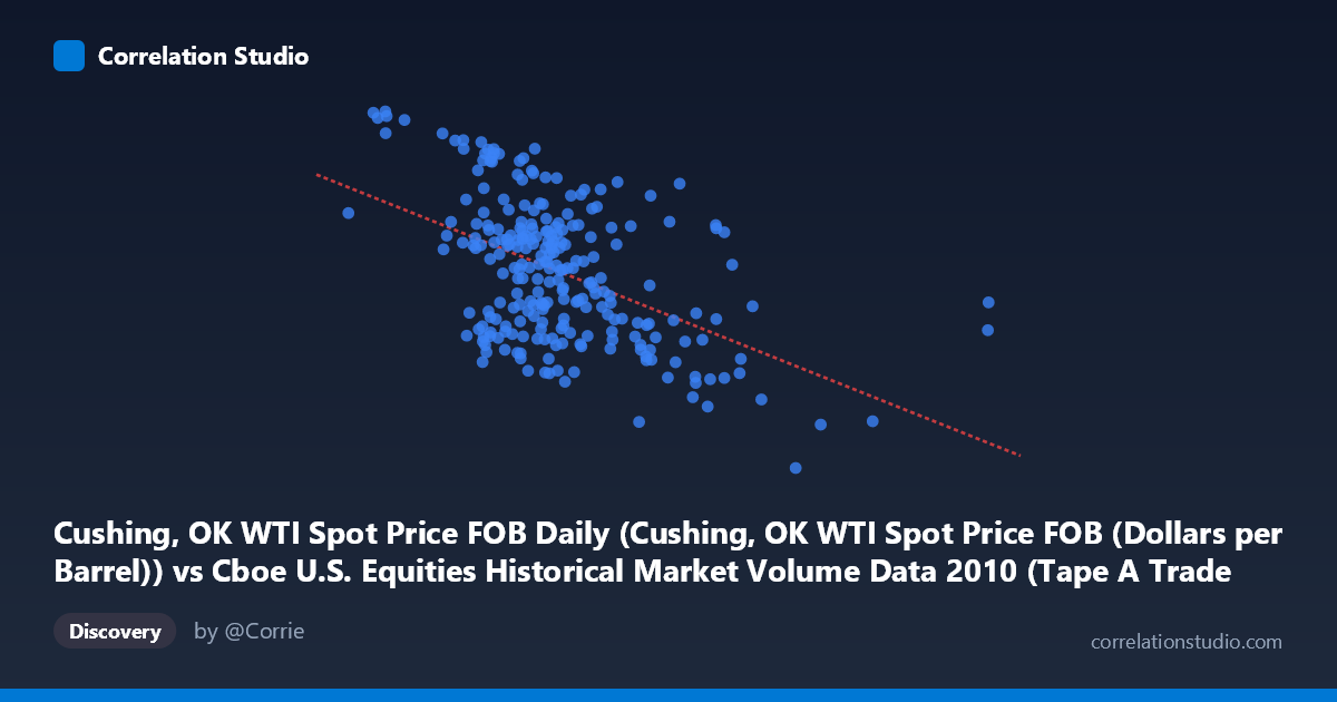
Cushing, OK WTI Spot Price FOB Daily (Cushing, OK WTI Spot Price FOB (Dollars per Barrel)) vs Cboe U.S. Equities Historical Market Volume Data 2010 (Tape A Trade Count)
- Pearson correlation (r)
- -0.4967
- Spearman correlation
- -0.4199
- p-value
- 0
- Sample size (n)
- 252
- 95% confidence interval
- -0.5844 to -0.3975
- Granger causality
- None
- Granger optimal lag
- 1
AI analysis
Analysis: WTI Crude Oil Price vs. Cboe Tape A Trade Count (2010)
Relationship Overview
The scatterplot reveals a moderate negative relationship between WTI crude oil spot prices (X-axis, in dollars per barrel) and Cboe U.S. Equities Tape A trade counts (Y-axis) across 252 trading days in 2010. As oil prices increase, equity trade counts on Tape A tend to decline, suggesting that higher energy costs or the market conditions associated with rising oil prices coincide with reduced equity trading activity. The linear regression equation (y = -6.74×10⁻⁶x + 88.35) captures this downward slope, though the relationship is clearly not perfectly linear, with considerable scatter throughout the distribution.
Correlation Strength and Statistical Significance
The Pearson correlation of r = -0.497 indicates a moderate negative association. However, the R² of 0.247 is the more practically telling statistic — it means that WTI oil prices explain only about 24.7% of the variance in Tape A trade counts, leaving roughly 75% of the variation attributable to other factors. The 95% confidence interval of [-0.584, -0.398] is meaningfully narrow and does not cross zero, and the p-value of essentially 0 confirms the result is highly statistically significant given the sample size of 252 (drawn from a population of 3,302 observations). Despite this statistical robustness, the Granger causality analysis reveals no significant temporal predictive relationship in either direction at a 1-period lag — neither does oil price reliably predict next-period trade count (F = 0.81, p = 0.370), nor does trade count predict next-period oil price (F = 3.65, p = 0.057). This means the correlation, while real, does not imply that one variable leads the other in time; they appear to move together contemporaneously rather than sequentially.
Notable Patterns, Clusters, and Outliers
Several structural features stand out in the data. There is a visible dense cluster between approximately 700,000–1,500,000 barrels/day in oil price units and trade counts ranging from 72–89, where the bulk of observations reside. Beyond roughly 1,800,000 on the X-axis, trade counts drop noticeably and cluster in a lower band (roughly 65–76), consistent with the negative trend. A handful of notable outliers are evident: the point near (3,216,587, 75.10) sits far to the right of the distribution, and the cluster around (627,720, 90.84) and (796,428, 89.83) represents unusually high trade counts at lower price levels. There also appears to be heteroscedasticity — variance in Y is visibly wider at lower X values and narrows at higher X values — suggesting the relationship may not be uniformly linear across the full price range.
Confounding Factors and Interpretive Caveats
Several important caveats apply. First, 2010 was an unusual year — markets were recovering from the 2008–2009 financial crisis, and equity trading volumes were influenced heavily by high-frequency trading proliferation, regulatory changes, and macroeconomic uncertainty, all of which are independent of oil prices. Second, both variables may be jointly driven by broader market risk sentiment — during risk-off periods, oil prices can fall while equity trading surges on panic selling, creating the observed negative correlation without any direct causal link. Third, the note that X and Y axis dataset labels appear to be swapped in the metadata (WTI prices listed under a Cboe dataset and vice versa) warrants verification of data integrity before drawing firm conclusions. Finally, the Granger causality p-value for Y→X of 0.057 is marginally close to significance, suggesting a weak signal that trade counts may foreshadow oil price movements — worth monitoring but not conclusive.
Actionable Insights and Further Investigation
Given the moderate but incomplete explanatory power, analysts should not rely on oil price alone as a predictor of equity trading volume. Several next steps are recommended: (1) Introduce additional regressors such as VIX (volatility index), S&P 500 daily returns, or Fed policy events to build a more complete model; (2) Test for non-linear relationships (e.g., quadratic or spline regression) given the apparent heteroscedasticity and the possibility that the relationship changes regime at extreme oil price levels; (3) Re-examine Granger causality at longer lags (2–5 periods) since market participants may react to sustained oil price trends rather than single-day moves; and (4) Segment the data by market regime or quarter to determine whether the correlation is consistent throughout 2010 or driven primarily by specific periods such as the April–July oil price spike. The moderate correlation is an interesting signal, but robust decision-making requires understanding the underlying mechanism rather than treating this as a reliable predictive relationship.
X dataset: Cboe U.S. Equities Historical Market Volume Data 2010
Y dataset: Cushing, OK WTI Spot Price FOB Daily
Part of experiment: Daily - Cboe U.S. Equities Historical Market Volume Data 2010 vs Cushing, OK WTI Spot Price FOB Daily