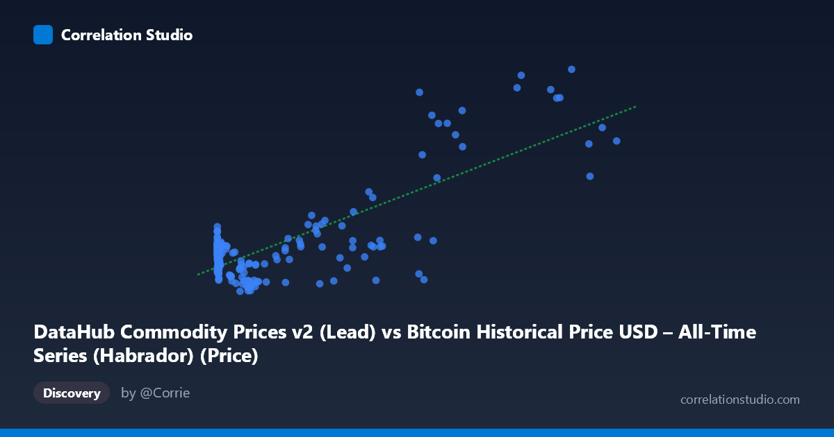
DataHub Commodity Prices v2 (Lead) vs Bitcoin Historical Price USD – All-Time Series (Habrador) (Price)
- Pearson correlation (r)
- 0.7875
- Spearman correlation
- 0.2449
- p-value
- 0
- Sample size (n)
- 182
- 95% confidence interval
- 0.725 to 0.837
- Granger causality
- None
- Granger optimal lag
- 4
- Time coverage
- 2010-08-01 to 2025-09-01
- Recomputed on refreshed data
- 2026-10-24 (r was 0.7875)
AI analysis
Analysis: Bitcoin Price vs. Commodity Price Index
1. Relationship Overview
The scatterplot displays a positive but distinctly non-linear relationship between Bitcoin's historical USD price (X-axis, spanning an enormous range from $0.06 to $113,500) and a commodity price series (Y-axis, ranging $64–$263). Because X spans nearly six orders of magnitude while Y varies within a much narrower band, the data is heavily compressed at low X-values and sparse at high X-values, giving the plot a classic "hockey-stick" or logarithmic-growth appearance rather than a clean linear scatter.
2. Strength, Direction, and Statistical Confidence
The correlation coefficient (r = 0.7875) indicates a strong positive linear association, with r² = 0.62 meaning the linear model explains about 62% of the variance in Y — leaving nearly 40% unexplained, likely due to the nonlinear scaling mismatch between the variables. The 95% CI [0.725, 0.837] is reasonably tight and excludes zero, and the p-value of 0 confirms this correlation is highly statistically significant and not due to chance, given n=182. However, statistical significance does not imply mechanistic causation. The Granger causality tests are telling: X→Y shows a borderline, non-significant result (F=2.42, p=0.0505), while Y→X shows no predictive power at all (p=0.64). This suggests neither series reliably predicts the other's future movements in a temporal/lagged sense, despite their strong contemporaneous correlation — a common signature of two trending time series that share an underlying time-based drift rather than a genuine causal link.
3. Notable Patterns and Outliers
Visually, low-X points (Bitcoin under ~$1,000, corresponding to 2010–2013) cluster tightly around Y≈85–110, showing modest commodity-price variation during Bitcoin's infancy. As X increases into the thousands and tens-of-thousands range (2017 onward), Y values spread more widely and trend upward, reaching the 120–260 range at the highest X values. Some notable outliers include points like (58724.66, 74.46) and (9148.44, 67.69), where high Bitcoin prices coincide with comparatively low commodity prices — likely reflecting temporary decoupling during Bitcoin-specific rallies or crashes (e.g., 2021–2022) that didn't align with broader commodity cycles. The extreme right-tail points (97365, 237.62) and (105620, 196.21) — near Bitcoin's all-time highs — pull the linear fit upward and disproportionately influence r² given their leverage.
4. Confounding Factors and Caveats
The most significant caveat is that both variables are essentially time-indexed series spanning 2010–2025, a period during which most assets — cryptocurrencies, equities, and commodities — experienced substantial secular inflation-driven or macro-driven price appreciation. This shared time trend is a classic confounder: any two upward-trending series will show spurious positive correlation without genuine economic linkage. Additionally, comparing Bitcoin's price in raw USD (which grew ~1,000,000×) against a bounded commodity index (which grew ~3×) is a scale mismatch that likely violates linear regression assumptions (homoscedasticity, linearity) — the model's residuals almost certainly show heteroscedastic patterns concentrated at low X-values.
5. Recommendations for Further Investigation
To draw more meaningful conclusions, it would be advisable to: (1) log-transform Bitcoin's price (given its exponential growth pattern) before re-running correlation/regression analysis, which may reveal a more linear and interpretable relationship; (2) detrend both series (e.g., using year-over-year returns rather than price levels) to test whether the correlation persists after removing shared temporal drift — this would better isolate genuine co-movement from spurious trend-driven correlation; (3) given the Granger results, avoid using this relationship for predictive/trading purposes, since neither series meaningfully leads the other; and (4) investigate whether a third variable (e.g., broad USD inflation, monetary policy, or overall risk-asset sentiment) better explains the shared upward trajectory of both series.
X dataset: Bitcoin Historical Price USD – All-Time Series (Habrador)
Y dataset: DataHub Commodity Prices v2
Part of experiment: Bitcoin - Bitcoin Historical Price USD – All-Time Series (Habrador) vs DataHub Commodity Prices v2