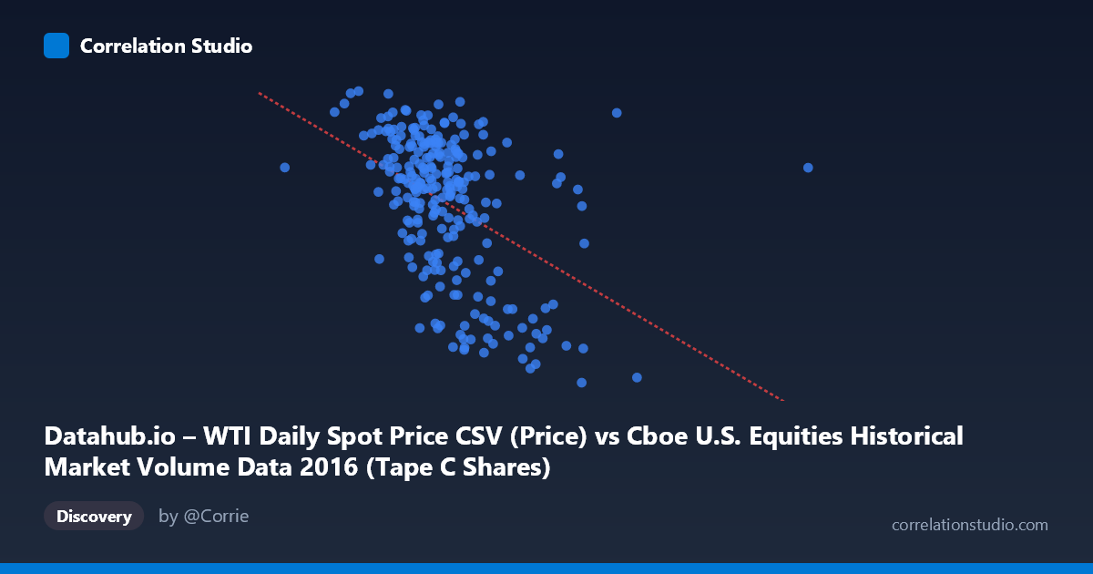
Datahub.io – WTI Daily Spot Price CSV (Price) vs Cboe U.S. Equities Historical Market Volume Data 2016 (Tape C Shares)
- Pearson correlation (r)
- -0.449
- Spearman correlation
- -0.4589
- p-value
- 0
- Sample size (n)
- 252
- 95% confidence interval
- -0.5425 to -0.3446
- Granger causality
- None
- Granger optimal lag
- 1
- Time coverage
- 2016-01-04 to 2016-12-30
- Recomputed on refreshed data
- 2026-10-23 (r was -0.449)
AI analysis
Scatterplot Analysis: WTI Crude Oil Price vs. Cboe Tape C Share Volume (2016)
Relationship Overview The scatterplot reveals a negative relationship between WTI crude oil daily spot prices (X-axis) and Cboe Tape C share volume (Y-axis) across 252 trading days in 2016. As oil prices increase, Tape C equity share volume tends to decrease, and vice versa. The linear regression equation (y = -1.11125E⁻⁰⁷x + 58.07) confirms this inverse slope, though the scatter around the regression line is substantial, suggesting the relationship is real but far from deterministic. Visually, the cloud of points shows a downward trend, with higher-volume days clustering at lower price levels and lower-volume days more dispersed across higher price ranges.
Correlation Strength and Statistical Significance The correlation coefficient of r = -0.449 indicates a moderate negative association. Crucially, the R² of 0.2016 means that only about 20% of the variance in Tape C share volume is explained by WTI price levels — leaving roughly 80% attributable to other factors. The 95% confidence interval of [-0.543, -0.345] is entirely negative, providing reasonable confidence that the true population correlation is genuinely inverse, not a sampling artifact. The p-value of 6.6×10⁻¹⁴ is overwhelmingly significant given n=252, making it statistically robust. However, the Granger causality tests reveal no significant temporal predictive direction in either direction (X→Y: F=1.57, p=0.211; Y→X: F=0.21, p=0.644), meaning that despite the concurrent correlation, neither variable's past values reliably predict the other's future values at a one-period lag. This important distinction separates statistical association from temporal forecasting utility.
Notable Patterns, Clusters, and Outliers Several features stand out in the data. There is a dense cluster of points in the X range of approximately 110–140 million (notional volume) and Y range of 43–51 ($/barrel), forming the core of the distribution. A secondary low-Y cluster appears at higher X values (roughly 140–175 million range), where oil prices fall into the high-20s to low-30s — likely corresponding to the early 2016 oil price trough when WTI briefly dipped below $30/barrel. Points like (175,021,320, 29.55) and (166,150,058, 33.21) stand as notable outliers representing extreme low-price, high-volume days. Conversely, some high-price days (near $51–54) cluster at relatively lower volume, consistent with the trend. The distribution appears somewhat heteroscedastic, with greater vertical spread at lower X values.
Confounding Factors and Interpretive Caveats Several important caveats apply. Macroeconomic context is critical — early 2016 was characterized by a global equity market selloff and oil price collapse simultaneously, meaning both variables may be driven by a common third factor (broad risk-off sentiment, global growth fears) rather than directly influencing each other. The Granger non-causality result reinforces this: the correlation may reflect co-movement driven by shared macro drivers rather than any causal mechanism. Additionally, Tape C specifically covers NYSE Arca-listed securities, which includes many energy-sector ETFs; during oil price stress, trading volumes in these instruments naturally spike, creating a mechanical link. The daily frequency also means short-term noise may inflate or obscure the underlying relationship. Finally, the population N of 3,622 vs. the sample n of 252 warrants caution — the sample covers one calendar year and may not generalize beyond 2016's specific market regime.
Actionable Insights and Further Investigation Given these findings, several avenues merit exploration. Segmenting the data by quarter would help isolate whether the correlation is driven primarily by the extreme Q1 2016 oil crash or persists throughout the year. Including a risk-sentiment proxy (e.g., VIX index) as a control variable would test whether the oil-volume relationship survives after accounting for broad market fear. Analysts should investigate whether energy-sector ETFs (e.g., XLE, USO) specifically drive Tape C volume during oil price moves, which would explain the mechanical link. Since Granger causality failed, vector autoregression (VAR) models with additional lags or multivariate controls could be tested before dismissing predictive utility entirely. Finally, extending the analysis to multiple years would determine whether 2016 represents an anomalous period or a recurring structural relationship between commodity markets and equity trading activity.
X dataset: Cboe U.S. Equities Historical Market Volume Data 2016
Y dataset: Datahub.io – WTI Daily Spot Price CSV
Part of experiment: Daily - Cboe U.S. Equities Historical Market Volume Data 2016 vs Datahub.io – WTI Daily Spot Price CSV