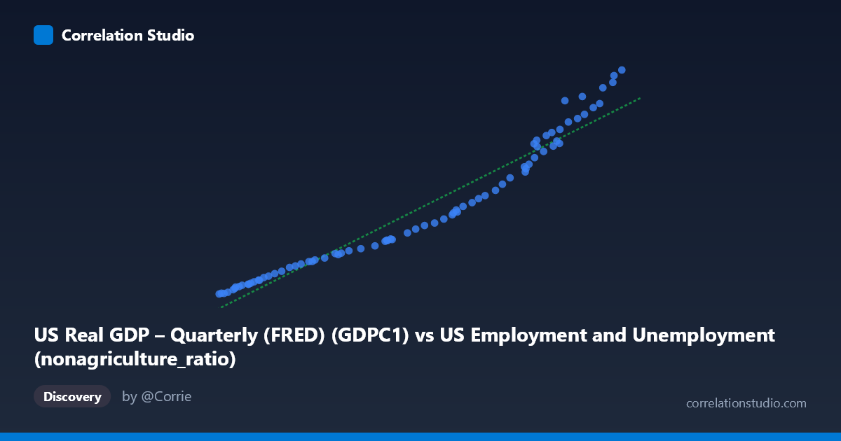
US Real GDP – Quarterly (FRED) (GDPC1) vs US Employment and Unemployment (nonagriculture_ratio)
- Pearson correlation (r)
- 0.9717
- Spearman correlation
- 0.9979
- p-value
- 0
- Sample size (n)
- 79
- 95% confidence interval
- 0.956 to 0.9819
- Granger causality
- None
- Granger optimal lag
- 10
- Time coverage
- 1947-01-01 to 2025-01-01
- Recomputed on refreshed data
- 2026-10-09 (r was 0.9719)
AI analysis
Analysis: US Real GDP vs. Non-Agriculture Employment Ratio
Relationship Overview
The scatterplot reveals a strong, positive, and nearly linear relationship between US Real GDP (quarterly, in billions of chained 2017 dollars) and the non-agriculture employment ratio. As GDP rises from roughly $49,000B to $161,000B, the non-agriculture ratio climbs correspondingly from approximately 2,183 to 23,548. The linear regression equation — y = 0.1721x − 7,696.71 — describes this trajectory well, with data points tracking closely along the fitted line across the full historical range from 1947 to 2025. This tight visual clustering around the regression line immediately signals an unusually strong co-movement between aggregate economic output and the structural composition of employment away from agriculture.
Correlation Strength and Statistical Significance
The correlation is exceptionally strong at r = 0.9719, and the coefficient of determination r² = 0.9446 means that approximately 94.5% of the variance in the non-agriculture employment ratio is statistically explained by variation in Real GDP. The 95% confidence interval for r is [0.9563, 0.9820], which is narrow and sits entirely in the high end of the correlation spectrum, indicating very low uncertainty about the strength of this association across repeated sampling. The p-value of effectively 0 confirms the relationship is not a statistical artifact. However, the Granger causality tests complicate the narrative: neither direction (X→Y: F=1.73, p=0.102; Y→X: F=1.69, p=0.111) reaches conventional significance at the 10% threshold. Despite the overwhelming cross-sectional correlation, neither variable reliably predicts the other's future values once lagged effects are accounted for at the optimal 10-period lag. This is a crucial caveat — high correlation does not imply temporal predictive power here.
Notable Patterns, Clusters, and Outliers
The data broadly divides into two loose visual regimes: a lower cluster (GDP < ~$80,000B, ratio < ~$6,000) representing the postwar era through roughly the early 1980s, characterized by denser point spacing, and an upper cluster (GDP ~$130,000B) representing the modern economy with wider scatter — suggesting slightly increasing variability at higher GDP levels, possibly a mild heteroscedastic pattern. A few points in the upper range (e.g., ~$145,446B paired with ~$20,709 and ~$161,268B with ~$23,548) appear to extend slightly above the central trend, hinting at periods where the non-agriculture share outpaced GDP growth. No dramatic outliers break from the pattern, but the rightmost observations deserve scrutiny as they reflect the most recent economic conditions and may embed post-pandemic labor market distortions.
Confounding Factors and Interpretive Caveats
Several important confounds limit causal interpretation. First, both variables share a common driver — long-run secular economic growth — meaning the correlation largely captures a shared time trend rather than a direct structural link. This is a textbook case of spurious correlation via common trend. Second, the agricultural-to-non-agricultural employment shift is a well-documented feature of economic development (structural transformation), meaning the relationship may reflect demographic and technological forces (mechanization, urbanization) rather than GDP per se. Third, the Granger non-causality result at 10 lags (~2.5 years) suggests the apparent predictive relationship dissolves once autocorrelation structure is properly modeled — neither series "leads" the other in a meaningful short-run sense. Finally, unit root and cointegration issues are highly likely given both series are non-stationary over 78 years, and standard r/r² statistics may be inflated as a result.
Actionable Insights and Further Investigation
Researchers should difference or detrend both series before drawing inferences, and formally test for cointegration (e.g., Engle-Granger or Johansen tests) to determine whether a genuine long-run equilibrium relationship exists beyond shared trending. If cointegration is confirmed, an Error Correction Model (ECM) would be more appropriate than the linear regression shown. It would also be valuable to segment the analysis by business cycle phases (expansions vs. recessions as dated by NBER) to examine whether the relationship weakens or reverses during downturns — the pandemic period in particular likely represents a structural break worth isolating. Additionally, incorporating productivity measures, sectoral wage data, or automation indices as controls could disentangle whether the GDP–employment composition link reflects demand-side growth or supply-side structural change, providing much richer policy-relevant insight.
X dataset: US Employment and Unemployment
Y dataset: US Real GDP – Quarterly (FRED)
Part of experiment: Yearly - US Employment and Unemployment vs US Real GDP – Quarterly (FRED)