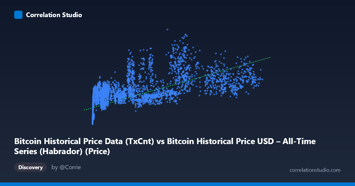
Bitcoin Historical Price Data (TxCnt) vs Bitcoin Historical Price USD – All-Time Series (Habrador) (Price)
- Pearson correlation (r)
- 0.673
- Spearman correlation
- 0.8701
- p-value
- 0
- Sample size (n)
- 5764
- 95% confidence interval
- 0.6586 to 0.6869
- Granger causality
- None
- Granger optimal lag
- 10
- Time coverage
- 2010-07-18 to 2026-04-28
AI analysis
Analysis: Bitcoin Transaction Count vs. Price
1. Relationship Overview
The scatterplot shows Bitcoin's daily transaction count (X) plotted against its USD price (Y) across nearly the full historical span (2010–2026). The data reveals a positive but clearly non-linear relationship: at low transaction counts (near-zero to a few thousand), prices span an enormous range (from under $1,000 to over $600,000 in the sample), while at higher transaction counts (50,000+), prices cluster more consistently in the $250,000–$650,000 range. This pattern—wide dispersion at low X, narrowing dispersion at high X—is a classic signature of a logarithmic or power-law relationship rather than a linear one, and it's consistent with the note that Spearman's ρ exceeds Pearson's r.
2. Strength, Direction, and Uncertainty
The linear Pearson correlation (r = 0.673) indicates a moderate-to-strong positive association, with R² = 0.453 meaning transaction count linearly explains only 45.3% of price variance—leaving over half unexplained by this single variable. The 95% CI [0.659, 0.687] is tight, and p ≈ 0 confirms the correlation is highly statistically significant given the large sample (n = 5,764)—essentially ruling out that this relationship arose by chance. However, statistical significance here reflects sample size more than practical predictive strength; nearly 55% of price movement is driven by other factors. Critically, the Granger causality tests show no significant predictive direction in either direction (X→Y: p = 0.994; Y→X: p = 0.369). This means neither variable's past values reliably help forecast the other's future values at the tested lag structure—the correlation appears to be a shared trend/co-movement (both rising over Bitcoin's history) rather than one causing or leading the other.
3. Notable Patterns and Outliers
Several structural features stand out: (a) early data points (very low X, low Y, e.g., X<20, Y<50,000) form a tight cluster representing Bitcoin's early years when both metrics were small; (b) a "fan" or funnel shape where variance in Y increases dramatically as X grows from near-zero to ~10,000, then the funnel narrows/plateaus after ~30,000 transactions; (c) some apparent outliers like (26930, 626942) and (58303, 656568) show high prices without correspondingly extreme transaction counts, suggesting periods of speculative price rallies decoupled from network usage growth (e.g., 2020-21 or 2024-25 bull markets driven by institutional/ETF demand rather than organic transaction growth). This non-linearity strongly suggests fitting log(X) or a power transformation would substantially improve model fit.
4. Confounding Factors and Caveats
This is time-series data where both variables are highly autocorrelated and trend upward over a 15+ year span—a textbook setup for spurious correlation via shared trend, rather than genuine mechanistic linkage. Bitcoin price is influenced by macroeconomic conditions, regulatory news, exchange listings, halving cycles, and speculative sentiment—none of which are captured by transaction count. Transaction count itself can be inflated by non-economic activity (e.g., batching, spam transactions, or protocol changes like SegWit/Lightning adoption that reduce on-chain transactions while usage grows). The lack of Granger causality reinforces that this is likely a coincidental co-trend rather than a causal price-driver relationship.
5. Suggestions for Further Investigation
Given the non-linear signal, refit using log-transformed X (or both variables) and compare R² improvement. De-trend both series (e.g., using differences or percentage changes) before re-testing correlation and Granger causality to control for the shared upward trend bias. Segment the analysis by market era (early/mid/bull-bear cycles) to see if the X-Y relationship is regime-dependent. Finally, incorporate additional covariates (active addresses, hash rate, macro indices like DXY or Nasdaq) to build a multivariate model, since transaction count alone explains less than half of price variance and shows no directional predictive power.
X dataset: Bitcoin Historical Price USD – All-Time Series (Habrador)
Y dataset: Bitcoin Historical Price Data
Part of experiment: Bitcoin - Bitcoin Historical Price USD – All-Time Series (Habrador) vs Bitcoin Historical Price Data