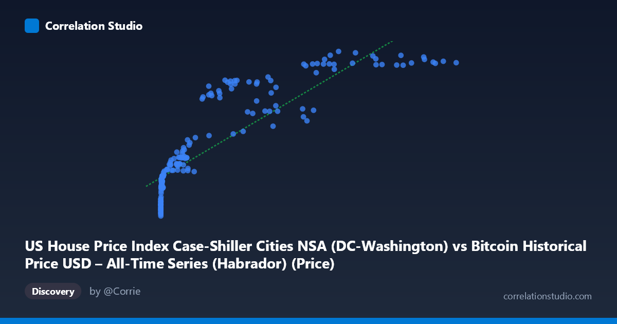
US House Price Index Case-Shiller Cities NSA (DC-Washington) vs Bitcoin Historical Price USD – All-Time Series (Habrador) (Price)
- Pearson correlation (r)
- 0.8666
- Spearman correlation
- 0.9703
- p-value
- 0
- Sample size (n)
- 187
- 95% confidence interval
- 0.8258 to 0.8984
- Granger causality
- None
- Granger optimal lag
- 1
AI analysis
Analysis: Bitcoin Price vs. US House Price Index (DC-Washington)
1. What the Visualization Reveals
The scatterplot shows a strong positive association between Bitcoin's historical price (X-axis) and the Case-Shiller Home Price Index for the Washington DC metro area (Y-axis). At low Bitcoin prices (under $1,000), the HPI clusters tightly in the 175–230 range. As Bitcoin climbs into the tens of thousands and beyond, the HPI rises correspondingly into the 280–340 range. However, the relationship is clearly curved, not linear — most of the meaningful HPI increase happens while Bitcoin moves from roughly $0 to $30,000, after which further Bitcoin gains (up to $118,670) produce comparatively modest additional HPI movement. This is a classic logarithmic/saturating pattern rather than a proportional one.
2. Strength, Direction, and Statistical Meaning
The Pearson correlation (r = 0.867, R² = 0.751) indicates a strong positive linear relationship, with the fitted line explaining about 75% of the variance in Y. The 95% CI [0.826, 0.898] is tight and excludes zero, and p ≈ 0 confirms this correlation is highly unlikely to be due to chance in-sample. However, the note that Spearman ρ exceeds Pearson r is the critical caveat: it signals the true relationship is monotonic but non-linear, meaning a log-transformed or polynomial fit would likely explain notably more variance than the 75.1% linear R² suggests. Importantly, the Granger causality tests show no significant predictive direction in either direction (X→Y: p=0.23; Y→X: p=0.11). This means neither series' past values help forecast the other's future values at the tested lag — the strong contemporaneous correlation is not evidence of a temporal lead-lag relationship. This is a crucial distinction: correlation here reflects two variables moving together over the same calendar period, not one driving the other.
3. Notable Patterns and Outliers
Several features stand out: - Dense low-end cluster: The vast majority of low-X points (Bitcoin under ~$1,000, largely pre-2017) sit in a narrow Y-band (180–220), reflecting Bitcoin's early years overlapping with a relatively flat post-2008-crash housing recovery period. - Compression/plateau at high X: Points like (85,197 → 339.4), (96,467 → 340.0), (105,920 → 335.8), (118,670 → 332.5) show HPI essentially plateauing or even slightly declining despite large continued increases in Bitcoin price — a strong sign of non-linearity/saturation. - Local dip anomaly: A cluster around X≈45,000–58,000 shows relatively lower Y-values (267–285) compared to neighboring higher-Y points at similar or lower X (e.g., 41,869→282.6 vs. 34,855→281.8 vs. 45,092→267.0), suggesting a temporary housing market pullback independent of Bitcoin's trajectory — likely a real 2022-type rate-driven housing correction. - No extreme outliers break the overall monotonic trend, but the shape clearly bends rather than following a straight line.
4. Confounding Factors and Caveats
This is almost certainly a spurious/confounded correlation driven by shared time trends rather than a causal economic relationship. Both series have risen substantially since 2010–2026, and any two upward-trending time series over the same period will show high correlation regardless of underlying mechanism (a classic "trending time series" statistical artifact). Real confounders likely include: broad macroeconomic conditions (low interest rates 2010–2021, pandemic-era stimulus, inflation surges), general asset-price/risk-appetite cycles, and secular growth in both crypto adoption and DC-area housing demand — none of which implies Bitcoin prices influence home values or vice versa. The lack of Granger causality reinforces that this is best understood as coincidental co-trending, not a functional relationship. Additionally, using raw (non-detrended) time series in correlation/regression inflates R² artificially — this is a well-known pitfall with non-stationary time series.
5. Suggestions for Further Investigation
1. Detrend or difference both series (e.g., use month-over-month % changes rather than levels) and re-run correlation — this will reveal whether any genuine relationship exists once shared time trends are removed. Expect the correlation to weaken substantially. 2. Fit a log(X) or polynomial model instead of linear, given the Spearman/Pearson discrepancy — this should improve explained variance and better represent the saturating shape. 3. Test cointegration (e.g., Engle-Granger or Johansen test) rather than relying on simple correlation, since both series are likely non-stationary trending series. 4. Control for common macro variables (interest rates, inflation, M2 money supply, or a stock market index) to see if the Bitcoin–HPI relationship persists or disappears — likely revealing both are driven by the same third factor. 5. Treat this correlation as descriptive/co-movement evidence only, not predictive or causal, given the Granger results — avoid using Bitcoin price as a forecasting input for DC housing prices (or vice versa) in any applied model.
X dataset: Bitcoin Historical Price USD – All-Time Series (Habrador)
Y dataset: US House Price Index Case-Shiller Cities NSA
Part of experiment: Bitcoin - Bitcoin Historical Price USD – All-Time Series (Habrador) vs US House Price Index Case-Shiller Cities NSA