Ethereum Historical Data (Daily) (IssTotNtv) vs Bitcoin Historical Price USD – All-Time Series (Habrador) (Price)
- Pearson correlation (r)
- -0.6987
- Spearman correlation
- -0.7111
- p-value
- 0
- Sample size (n)
- 3926
- 95% confidence interval
- -0.7144 to -0.6823
- Granger causality
- None
- Granger optimal lag
- 10
AI analysis
Analysis: Ethereum Issuance/Transaction Metric vs. Bitcoin Price
1. Overview of the Relationship
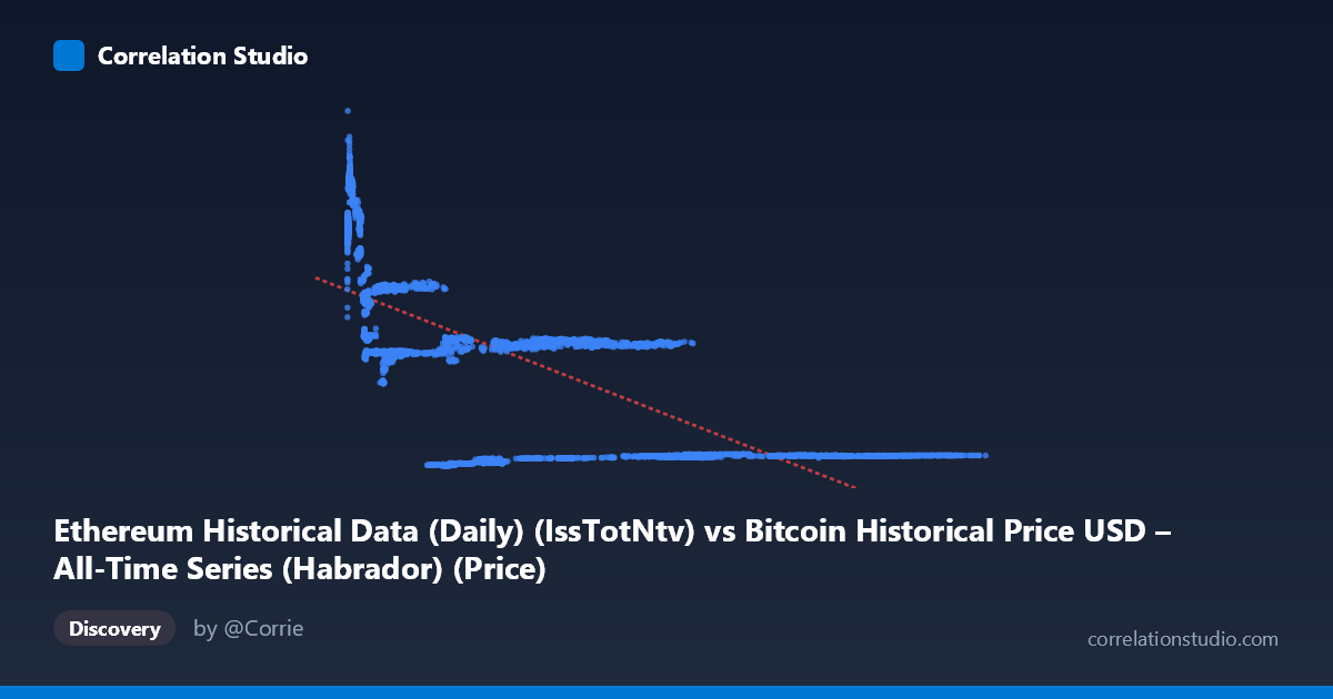
The scatterplot reveals a clear negative, non-linear relationship between the two variables. Rather than a uniform linear decline, the data forms distinct clusters at different X-value ranges: a dense cluster of high-Y values (13,000–20,000+) concentrated at low X (roughly 200–20,000), a mid-range cluster around Y≈14,000–15,000 spanning X from ~20,000–50,000, and a sparse tail of low-Y values (~2,500–2,700) at high X (~40,000–120,000). This suggests the relationship may be better characterized as a step-like or threshold decay rather than a smooth linear trend, with Y values dropping sharply once X exceeds certain ranges.
2. Strength, Direction, and Statistical Confidence
The correlation coefficient (r = -0.6987, r² = 0.4882) indicates a moderately strong negative relationship, with the linear model explaining 48.8% of the variance in Y — meaning over half the variability remains unexplained by X alone, consistent with the clustered, non-linear pattern observed visually. The 95% CI [-0.7144, -0.6823] is tight and the p-value is effectively 0, confirming this correlation is highly statistically significant and not a product of sampling noise, even though the practical explanatory power is capped at moderate levels. Critically, the Granger causality tests show no significant predictive direction in either direction (X→Y: p=0.69; Y→X: p=0.46), meaning past values of one series do not meaningfully forecast future values of the other. This is an important caveat: despite the strong static correlation, there is no evidence of temporal lead-lag causality — the relationship appears contemporaneous/structural rather than dynamically predictive.
3. Notable Patterns and Outliers
Several structural features stand out: - Distinct horizontal bands: Y clusters near 2,500–2,700 (high X), ~13,000–15,000 (low-to-mid X), and ~18,000–32,000 (very low X, under ~10,000). This banding suggests underlying regime changes or discrete states rather than continuous covariation. - A curved upper-left arm: as X approaches its minimum (~200–1,000), Y spikes to its maximum (27,000–32,000+), suggesting a possible inverse power-law or exponential decay curve rather than a straight line. - Low-X, low-Y outliers: e.g., (16552.57, 1702.40) and (21788.20, 1806.14) break from the mid-range cluster, indicating some volatility or additional structure not captured by X alone.
4. Confounding Factors and Caveats
Given the metadata, there appears to be a column/label mismatch — X is described as an Ethereum issuance/transaction metric while Y is labeled Bitcoin price, but the dataset descriptions reference cross-linked, possibly misaligned sources. This raises concerns about data integrity and variable definition that should be resolved before drawing causal conclusions. Additionally, both cryptocurrencies are known to be driven by shared macro factors (market sentiment, regulatory news, liquidity cycles), meaning the correlation may reflect common external drivers rather than a direct mechanical relationship. The long time span (2015–2026) also spans multiple bull/bear cycles, and clustering suggests regime-dependent behavior — the relationship may only hold within certain market phases, inflating the overall r when pooled.
5. Recommendations for Further Investigation
1. Verify data labeling/alignment — confirm that X and Y columns are correctly mapped to their stated definitions and time-synchronized. 2. Segment by market regime or time period (e.g., bull vs. bear cycles) to test whether the negative correlation holds consistently or is driven by a few structural breaks. 3. Explore non-linear models (log-log, piecewise regression, or spline fitting) given the visual clustering and curved tail, which likely outperform the linear fit (r²=0.488). 4. Investigate common confounders (e.g., overall crypto market cap, BTC dominance index) using multivariate regression to isolate whether this bivariate relationship is direct or spurious. 5. Given the lack of Granger causality, avoid using either series to forecast the other in trading strategies; treat the correlation as descriptive/structural rather than predictive.
X dataset: Bitcoin Historical Price USD – All-Time Series (Habrador)
Y dataset: Ethereum Historical Data (Daily)
Part of experiment: Bitcoin - Bitcoin Historical Price USD – All-Time Series (Habrador) vs Ethereum Historical Data (Daily)