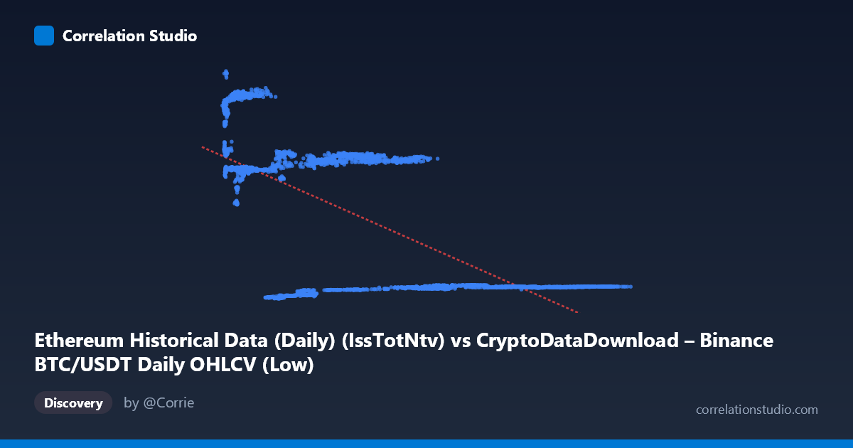
Ethereum Historical Data (Daily) (IssTotNtv) vs CryptoDataDownload – Binance BTC/USDT Daily OHLCV (Low)
- Pearson correlation (r)
- -0.6435
- Spearman correlation
- -0.4764
- p-value
- 0
- Sample size (n)
- 3191
- 95% confidence interval
- -0.6634 to -0.6227
- Granger causality
- None
- Granger optimal lag
- 10
- Time coverage
- 2017-08-17 to 2026-05-20
AI analysis
Analysis of the X–Y Relationship
Note on data labeling: The column headers appear mismatched — the X-axis is labeled as an Ethereum issuance metric but the description points to BTC/USDT OHLCV data, and Y is labeled as a Binance "Low" price but described as Ethereum network metrics. The values themselves (X ranging ~2,800–123,000; Y ranging ~1,550–22,700) look like they could plausibly be price or volume-scale figures rather than gas/transaction counts. For this analysis, I'll treat X and Y purely as the two numeric series provided, since the metadata conflict makes the "true" identity of the variables unreliable.
1. What the Scatterplot Reveals
The data shows a clear negative, non-linear relationship that resembles a step-function or clustered pattern more than a smooth linear decline. Looking at the sample points, there appear to be distinct horizontal bands in Y (~2,000–2,800, ~13,400–14,900, ~18,500–21,000) that each correspond to specific ranges of X. This suggests the relationship may be driven by regime shifts or discrete categories rather than continuous covariation — low X values associate with high Y values (13,000–21,000), while high X values (50,000) consistently pull Y down to 2,000–2,900.
2. Strength, Direction, and Uncertainty
The correlation coefficient (r = -0.6435, R² = 0.414) indicates a moderate-to-strong negative relationship, with about 41% of the variance in Y statistically explained by X — leaving the majority (59%) unexplained, likely due to the clustering/regime behavior noted above rather than pure noise. The narrow 95% CI [-0.6634, -0.6227] combined with p ≈ 0 (and n = 3,191) means this correlation is highly statistically reliable and not a sampling artifact — we can be confident the linear association is real and consistently negative across the dataset.
However, the Granger causality results are important: neither variable significantly predicts the other in a temporal/lagged sense (X→Y: p = 0.76; Y→X: p = 0.051, only marginally short of significance). This tells us the strong contemporaneous correlation is not evidence of one variable driving the other over time — it may instead reflect both variables reacting to a shared external driver, or a structural/definitional relationship (e.g., if one is partially derived from or bounded by the other).
3. Notable Patterns and Outliers
The most striking feature is the banding: Y values cluster tightly around 2,000–2,800, 13,400–14,900, and 18,500–21,000, with little continuous spread between these bands. This is inconsistent with a simple linear model and suggests either (a) discretized/categorical underlying data, (b) regime-dependent behavior (e.g., market cycles, bull/bear phases), or (c) an artifact of merging two datasets with different native granularities. The linear regression line (y = -0.139x + 15,240) is a poor descriptor of this banded structure — it will systematically over/under-predict within each cluster.
4. Confounding Factors and Caveats
Several caveats apply: - Metadata mismatch: the column descriptions don't match the axis labels, raising concern about how X and Y were joined/aligned (possibly a mismatched timestamp merge across two different source datasets and assets, BTC vs. ETH). - Time-series autocorrelation: both series likely have strong internal trends/momentum (typical of price or on-chain crypto metrics), which can inflate simple correlation without implying a genuine bivariate relationship — a classic spurious correlation risk in time series. - Non-stationarity: crypto price/volume data over 2017–2026 spans multiple bull/bear cycles; correlation calculated over pooled non-stationary data can be an artifact of shared trend rather than true dependence. - Non-linear/clustered structure: as noted, R²=0.41 from a linear fit likely understates or misrepresents the true (possibly step-like or threshold-based) relationship.
5. Suggested Next Steps
1. Verify data provenance — confirm the actual identity and correct temporal alignment of X and Y before drawing substantive conclusions. 2. Test stationarity (e.g., ADF test) and consider differencing or working with returns/log-changes rather than levels, then re-run correlation and Granger tests to rule out spurious trend-driven correlation. 3. Investigate the banding — cluster the data (e.g., k-means or regime-detection) to see if distinct regimes/eras explain the discrete Y bands, and consider a piecewise or non-linear model (e.g., quantile regression, decision tree) instead of simple linear regression. 4. Explore lagged cross-correlation more finely (shorter/longer lags) since Y→X was borderline significant (p=0.051) — a finer lag search might reveal a real but weak predictive signal. 5. Add a third variable/control (e.g., overall market cap, time trend) to check whether the negative correlation persists after controlling for shared macro trends — this would help distinguish genuine dependency from confounded co-movement.
X dataset: CryptoDataDownload – Binance BTC/USDT Daily OHLCV
Y dataset: Ethereum Historical Data (Daily)
Part of experiment: Bitcoin - CryptoDataDownload – Binance BTC/USDT Daily OHLCV vs Ethereum Historical Data (Daily)