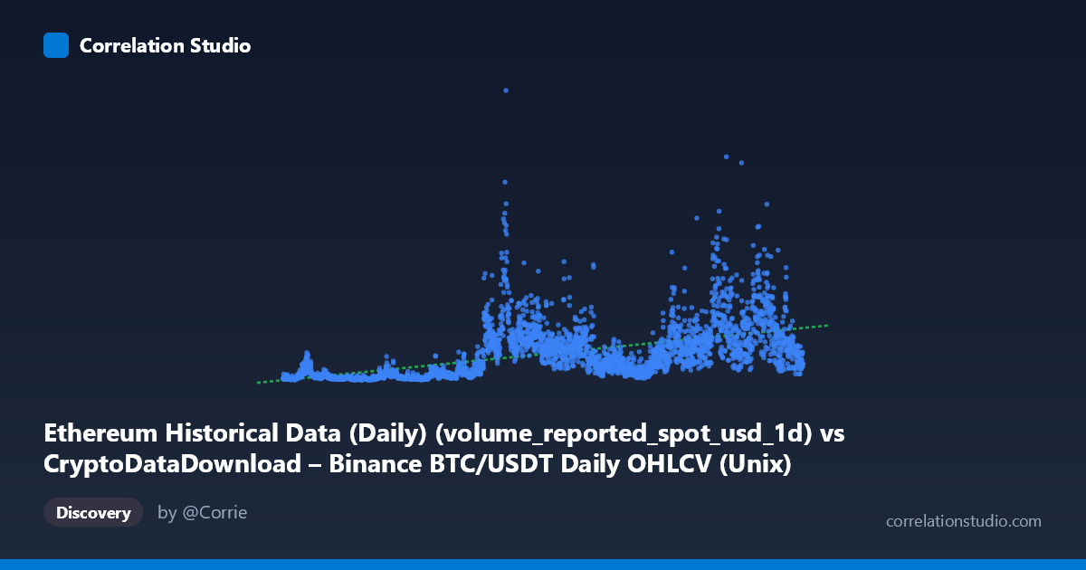
Ethereum Historical Data (Daily) (volume_reported_spot_usd_1d) vs CryptoDataDownload – Binance BTC/USDT Daily OHLCV (Unix)
- Pearson correlation (r)
- 0.5382
- Spearman correlation
- 0.7032
- p-value
- 0
- Sample size (n)
- 3191
- 95% confidence interval
- 0.5131 to 0.5624
- Granger causality
- Y → X
- Granger optimal lag
- 10
- Time coverage
- 2017-08-17 to 2026-05-20
AI analysis
Analysis: BTC Trading Volume vs. Ethereum Timestamp Metric
Note on data labeling: The axis metadata appears mismatched — X is described as Ethereum volume while Y is labeled as a Binance BTC/USDT Unix timestamp, but the actual values (Y ranging from ~$100M to $53B) strongly suggest Y is actually a volume or market metric, not a timestamp, and X (given its range of ~1.5–1.78 trillion) is functioning as a time index (likely Unix milliseconds representing dates from 2017–2026). This analysis proceeds treating X as a time axis and Y as a volume/value metric, consistent with the sample data pattern.
1. What the Visualization Reveals The scatterplot shows a time-series-like relationship where Y (volume) fluctuates substantially across the observation period (2017–2026), with values ranging from ~$107M to ~$53.6B. Rather than a clean linear trend, the data shows clustering at lower values (hundreds of millions to low billions) in earlier periods (2017–2020) and increasing dispersion with higher peaks (multi-billion dollar spikes) in later periods (2021 onward), suggesting growing market volume and volatility over time.
2. Strength, Direction, and Statistical Confidence The Pearson correlation (r = 0.538) indicates a moderate positive relationship, with R² = 0.290 meaning only 29% of the variance in Y is explained by X — the majority (71%) is driven by other factors. The 95% CI [0.513, 0.562] is tight and the p-value ≈ 0 confirms this correlation is highly statistically significant and not due to chance, given the large sample (n=3,191). However, statistical significance here reflects the large N more than practical predictive strength — a moderate r² means X alone is a weak-to-moderate predictor of Y.
The Granger causality results are particularly noteworthy: Y Granger-causes X (F=2.06, p=0.024) but not vice versa (p=0.212). This suggests that past values of Y have predictive power for future X values at a 10-period lag, while X does not help predict Y. This is an important asymmetry — it implies the "volume" variable (Y) may be a leading indicator for whatever X represents, rather than the reverse.
3. Notable Patterns and Outliers The sample data shows clear volatility clustering: values in 2017–2019 are consistently low (~$200M–$700M), while 2021–2025 show dramatic spikes exceeding $10B–$19B (e.g., 1741564800000 → $18.98B, 1642723200000 → $14.59B). This pattern is consistent with crypto market cycles (bull/bear phases) rather than steady linear growth. The mention that Spearman ρ Pearson r signals a monotonic but non-linear relationship — likely logarithmic or exponential, common in financial volume data which often grows multiplicatively rather than additively. A log-transform of Y would likely improve model fit substantially.
4. Confounding Factors and Caveats Given the metadata confusion, a key caveat is data provenance clarity — confirming what X and Y actually represent is critical before drawing market conclusions. Beyond that, both series likely share common macro drivers (crypto market cycles, BTC/ETH price correlation, regulatory events, exchange listings) that could inflate correlation without direct causal linkage. Volume-based crypto metrics are also prone to exchange-specific reporting anomalies, wash trading, and API/data gaps, which could introduce noise or artificial spikes untied to genuine market behavior.
5. Suggested Next Steps 1. Verify axis semantics — confirm actual variable identities before further modeling. 2. Apply log or Box-Cox transformation to Y (and possibly X) to test whether R² improves, given the Spearman/Pearson divergence. 3. Investigate the Granger-causal lag structure (10 periods) further — test shorter lags and consider whether this reflects a genuine leading indicator relationship or an artifact of shared trend/seasonality. 4. Segment by market regime (bull vs. bear phases) to check if correlation strength is regime-dependent rather than constant. 5. Control for shared trend by differencing both series (returns/changes rather than levels) to reduce spurious correlation from co-trending non-stationary time series — this is especially important given both variables show strong upward drift over time.
X dataset: CryptoDataDownload – Binance BTC/USDT Daily OHLCV
Y dataset: Ethereum Historical Data (Daily)
Part of experiment: Bitcoin - CryptoDataDownload – Binance BTC/USDT Daily OHLCV vs Ethereum Historical Data (Daily)