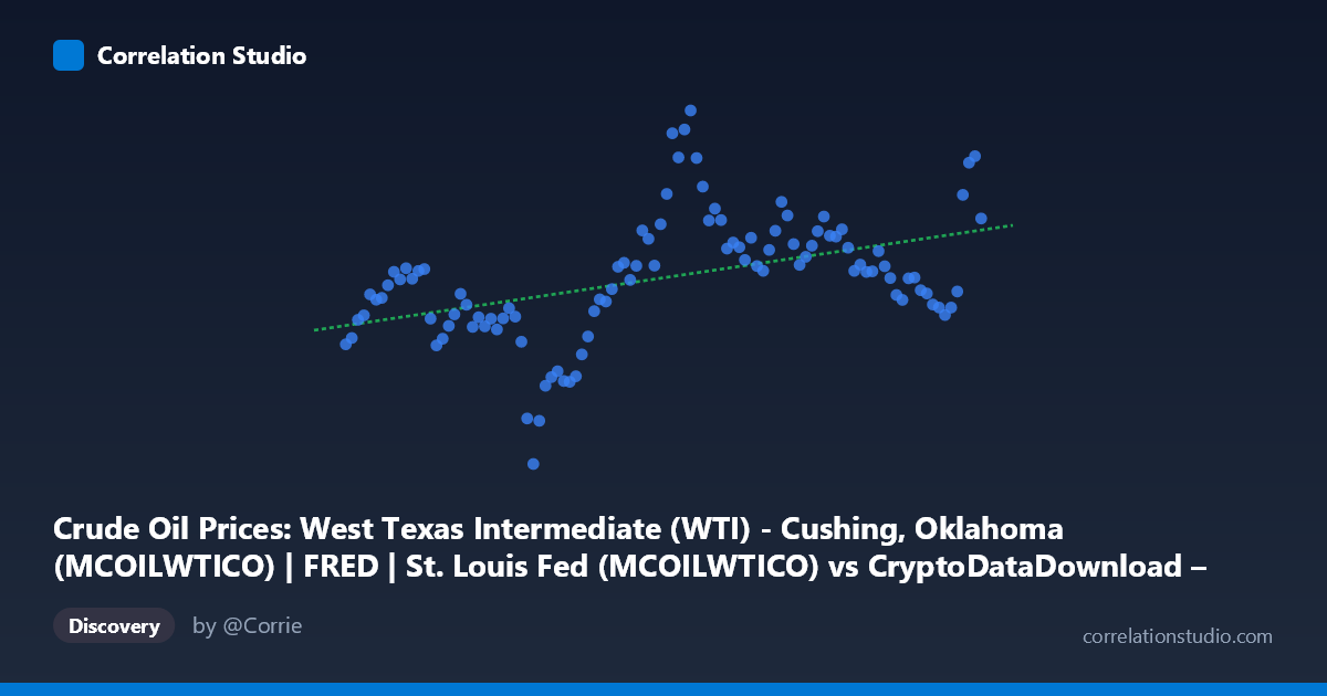
Crude Oil Prices: West Texas Intermediate (WTI) - Cushing, Oklahoma (MCOILWTICO) | FRED | St. Louis Fed (MCOILWTICO) vs CryptoDataDownload – Binance BTC/USDT Daily OHLCV (Unix)
- Pearson correlation (r)
- 0.4501
- Spearman correlation
- 0.5191
- p-value
- 0.000001
- Sample size (n)
- 106
- 95% confidence interval
- 0.2837 to 0.5902
- Granger causality
- None
- Granger optimal lag
- 8
AI analysis
Analysis: WTI Crude Oil Prices vs. Time (Mislabeled Axes)
Important preliminary note: The axis labels appear swapped or mismatched in the metadata. The X-axis is described as timestamps (ranging 2017–2026) but labeled as WTI crude oil prices, while Y-axis values (16.55–114.84) look like actual oil prices in USD/barrel, not Unix timestamps. Based on the data itself, this appears to be a time series of WTI crude oil prices from 2017 to 2026, and the "correlation" being measured is essentially price vs. time (trend), not a relationship between two independent economic variables like BTC and oil. The analysis below treats X as time and Y as WTI price, which matches the actual data pattern.
1. What the Visualization Reveals
The scatterplot shows WTI crude oil prices plotted against time from September 2017 to June 2026. The data reveals a moderate upward drift in price over this period, punctuated by significant volatility. Prices start in the $60s, crash dramatically to near $16.55 in early-to-mid 2020 (consistent with the COVID-19 demand shock and negative-pricing event), then recover and trend generally higher, reaching values above $100 in later periods (2025–2026 sample points).
2. Strength, Direction, and Statistical Confidence
The correlation coefficient (r = 0.45) indicates a moderate positive relationship between time and price, but r² = 0.203 tells the more important story: only ~20% of the variance in oil prices is explained by the linear time trend. The remaining 80% is driven by other factors (supply shocks, geopolitical events, demand cycles, etc.), meaning a simple linear model is a weak predictor of price at any given point in time.
The 95% CI [0.284, 0.590] is reasonably tight and entirely positive, and the p-value (1.29E-06) is highly significant — so we can be confident a real, non-zero upward trend exists across the full population (N=486). However, statistical significance here reflects the large sample size and long time span, not necessarily practical predictive power, given the modest r².
The Granger causality results are essentially a formality here since X is time itself — time cannot be "caused" by price, and the lack of significant bidirectional causality (p = 0.071 and p = 0.222) simply confirms there's no meaningful lagged feedback structure between the (likely mislabeled) series, reinforcing that this is a straightforward trend analysis rather than a dynamic two-variable system.
3. Notable Patterns and Outliers
Several features stand out: - A sharp trough in Q1–Q2 2020 (values near 16–17), corresponding to the COVID-19 oil price collapse — this is a major outlier/structural break, not part of a smooth trend. - A secondary peak in 2022 (~109), aligning with post-pandemic recovery and the Russia-Ukraine war supply disruption. - A strong rally into 2025–2026 (values 85–102+), suggesting renewed upward momentum or a new demand/supply regime. - The data is not linear — it resembles a series of regime shifts (crash, recovery, spike, plateau, rally) rather than steady growth, which explains why the linear r² is capped at ~20%.
4. Confounding Factors and Caveats
- Axis mislabeling: The dataset descriptions suggest BTC/USDT OHLCV data was cross-referenced with WTI prices, but the actual X/Y values don't match those descriptions — this needs to be resolved before drawing economic conclusions about BTC-oil linkage. - Non-stationarity: Oil prices exhibit trends, volatility clustering, and structural breaks (2020 crash, 2022 spike) that violate assumptions of simple linear correlation/Granger tests. - Autocorrelation: Time series data is highly autocorrelated, which can inflate apparent significance in naive correlation tests. - External shocks (pandemic, war, OPEC+ decisions) are omitted variables driving most of the price variance not captured by a time trend.
5. Suggested Next Steps
1. Verify and correct axis labels/data mapping — confirm whether this is meant to be BTC price vs. WTI price (a genuine cross-asset correlation) rather than WTI vs. time. 2. If BTC vs. WTI is the intended analysis, re-run correlation using actual BTC closing prices against WTI, ideally with returns (% change) rather than levels, to avoid spurious trend-driven correlation. 3. Apply piecewise or regime-switching models (e.g., segmenting around 2020 and 2022 shocks) rather than a single linear fit, given the visible structural breaks. 4. Test for stationarity (ADF test) and consider differencing the series before any causality testing, since Granger causality assumes stationary inputs. 5. Investigate specific event windows (COVID crash, 2022 energy crisis) as case studies rather than relying solely on aggregate correlation statistics.
X dataset: CryptoDataDownload – Binance BTC/USDT Daily OHLCV
Y dataset: Crude Oil Prices: West Texas Intermediate (WTI) - Cushing, Oklahoma (MCOILWTICO) | FRED | St. Louis Fed
Part of experiment: Bitcoin - CryptoDataDownload – Binance BTC/USDT Daily OHLCV vs Crude Oil Prices: West Texas Intermediate (WTI) - Cushing, Oklahoma (MCOILWTICO) | FRED | St. Louis Fed