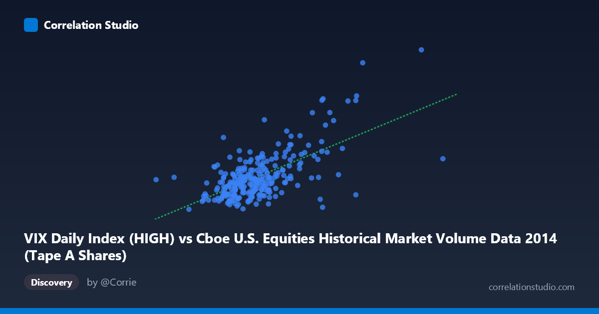
VIX Daily Index (HIGH) vs Cboe U.S. Equities Historical Market Volume Data 2014 (Tape A Shares)
- Pearson correlation (r)
- 0.6358
- Spearman correlation
- 0.5197
- p-value
- 0
- Sample size (n)
- 252
- 95% confidence interval
- 0.5558 to 0.704
- Granger causality
- None
- Granger optimal lag
- 1
AI analysis
Scatterplot Analysis: VIX Daily Index (HIGH) vs. Tape A Shares Volume
Relationship Overview
The scatterplot reveals a moderate positive relationship between Cboe VIX Daily Index High values and Tape A Shares trading volume across 2014 U.S. equity markets. As VIX High readings increase, Tape A share volume tends to rise correspondingly, which aligns well with established market intuition: elevated volatility environments typically attract higher trading activity as investors hedge positions, rebalance portfolios, or react to market stress events. The linear regression equation (y = 4.17×10⁻⁸x + 5.33) confirms this positive slope, though the intercept suggests a meaningful baseline volume level even during calm market periods.
Correlation Strength and Statistical Significance
The correlation coefficient of r = 0.636 indicates a moderately strong positive association, with r² = 0.404 meaning that approximately 40.4% of the variance in Tape A share volume is explained by VIX High readings — a meaningful but far from complete explanatory relationship. The remaining ~60% of variance stems from other factors entirely. The 95% confidence interval [0.556, 0.704] is reassuringly narrow given the sample of n = 252 paired observations drawn from a population of N = 3,686, and the p-value of effectively zero confirms this relationship is not attributable to random chance. However, the Granger causality analysis tells a critical story: neither direction (X→Y: F = 1.42, p = 0.235; Y→X: F = 0.26, p = 0.608) reaches statistical significance at conventional thresholds. This means that despite a robust contemporaneous correlation, neither variable reliably predicts the other one period ahead, cautioning strongly against any causal or forecasting interpretation.
Notable Patterns, Clusters, and Outliers
Several structural features are visible in the sample data. The bulk of observations cluster in a moderate-volatility, moderate-volume zone (VIX High roughly 11–18, volume in the 150M–280M range), consistent with the relatively calm first half of 2014. However, there are notable high-leverage outliers — most prominently points near (362M, 29.4) and (355M, 25.2) — where both volume and VIX spike simultaneously, likely corresponding to discrete market stress episodes (e.g., geopolitical events or October 2014 equity selloff). The point at (312M, 11.0) stands out as an anomaly with very high volume but unusually low VIX, suggesting that elevated volume can occur in low-volatility conditions, potentially during index rebalancing or expiration events. This heteroscedasticity — variance in Y increasing at higher X values — hints that a linear model may underfit the tail behavior.
Confounding Factors and Caveats
Several important caveats apply. First, the axes appear to be swapped from their natural causal direction: VIX is conventionally the dependent response to market conditions, not a predictor of volume, yet here VIX High is plotted on X. Second, both variables are likely jointly driven by common underlying factors — macroeconomic news releases, Federal Reserve policy announcements, earnings seasons, and end-of-month/quarter rebalancing flows — making the observed correlation partly spurious. Third, intraday timing mismatches may exist since VIX High represents a within-day extreme while Tape A shares reflects total daily volume, introducing measurement asymmetry. Finally, 2014 represents a single, relatively benign market year; the relationship may behave quite differently in crisis years (2008, 2020) where VIX ranges expand dramatically.
Actionable Insights and Further Investigation
Practitioners and researchers should consider several next steps. A regime-segmented analysis (low/medium/high VIX terciles) would test whether the linear relationship holds uniformly or is driven primarily by high-stress tail observations. Introducing additional covariates such as S&P 500 returns, options expiration calendars, and Fed meeting dates through multiple regression would likely substantially increase explained variance beyond the current 40%. Given the absence of Granger causality, same-day simultaneous modeling (structural equation modeling or VAR with contemporaneous terms) is more appropriate than lag-based forecasting. Finally, extending the analysis across multiple years — particularly including 2008, 2015–2016, and 2020 — would clarify whether this correlation is a stable structural feature of U.S. equity markets or an artifact of 2014's specific volatility environment.
X dataset: Cboe U.S. Equities Historical Market Volume Data 2014
Y dataset: VIX Daily Index
Part of experiment: Daily - Cboe U.S. Equities Historical Market Volume Data 2014 vs VIX Daily Index