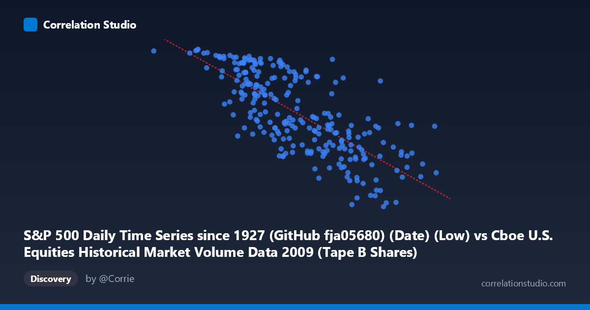
S&P 500 Daily Time Series since 1927 (GitHub fja05680) (Date) (Low) vs Cboe U.S. Equities Historical Market Volume Data 2009 (Tape B Shares)
- Pearson correlation (r)
- -0.7527
- Spearman correlation
- -0.7624
- p-value
- 0
- Sample size (n)
- 252
- 95% confidence interval
- -0.8017 to -0.6936
- Granger causality
- Bidirectional
- Granger optimal lag
- 10
AI analysis
Scatterplot Analysis: S&P 500 Daily Low vs. Cboe Tape B Shares Volume (2009)
Relationship Overview
The scatterplot reveals a clear negative relationship between the S&P 500 daily low price (X-axis) and Cboe Tape B share volume (Y-axis) across the 2009 trading year. As the S&P 500's daily low increases — reflecting price recovery throughout the year — Tape B share volume systematically declines. This pattern is visually coherent with a downward-sloping linear trend, captured by the regression equation y = -2.07 × 10⁻⁶x + 1,242.47, meaning that for every ~483 million unit increase in the daily low, Tape B volume decreases by approximately one unit. The data spans a wide X range (~34M to ~256M in index units), reflecting the dramatic market recovery from the March 2009 lows to year-end highs, providing a natural quasi-experiment in how trading behavior responds to equity price levels.
Correlation Strength, Direction, and Causality
The correlation coefficient of r = -0.753 indicates a moderately strong negative linear association. More meaningfully, r² = 0.567 tells us that roughly 56.7% of the variance in Tape B share volume is explained by the S&P 500 daily low — a substantial explanatory share for financial market data, though nearly 43% of variance remains unaccounted for. The 95% confidence interval of [-0.802, -0.694] is notably tight and entirely negative, providing strong statistical confidence that the inverse relationship is real and not an artifact of sampling. The p-value of effectively zero, combined with N = 3,232, leaves no reasonable doubt about statistical significance. Granger causality testing adds a temporal dimension: bidirectional Granger causality is detected at an optimal lag of 10 periods, with both X→Y (F = 2.44, p = 0.009) and Y→X (F = 2.77, p = 0.003) being significant. This suggests that neither price levels nor volume are strictly exogenous — past S&P lows help predict future Tape B volume, and past volume helps predict future price lows, consistent with the well-documented price-volume feedback loop in equity markets.
Notable Patterns, Clusters, and Outliers
Several structural features stand out in the scatter. There is a visible concentration of high-volume, low-price points in the lower-left region of the plot (e.g., the point near X ≈ 33.8M, Y ≈ 1,121 and X ≈ 66.8M, Y ≈ 1,122), likely corresponding to the early 2009 crisis period when the S&P 500 was near its March lows and fear-driven volume was elevated. Conversely, the upper-right region is sparsely populated, representing late-2009 recovery periods with lower relative volume. A few apparent outliers exist — notably the point near (254.5M, 901) and (225.7M, 909), which show higher-than-expected volume for elevated price levels, potentially reflecting specific high-activity trading sessions or index rebalancing events. The scatter also shows increased dispersion at intermediate price levels, suggesting the linear model is a reasonable but imperfect fit, and that volatility regimes modulate the price-volume relationship non-uniformly across the year.
Confounding Factors and Caveats
Several important caveats temper this analysis. First, 2009 is a highly anomalous year — the post-financial crisis recovery represents an extreme regime that may not generalize to normal market conditions. The negative correlation may be largely a spurious temporal artifact: both variables are time-indexed, and as calendar time progresses, prices rose (recovery) while elevated crisis-period volume gradually normalized, meaning the correlation may reflect shared trends rather than a structural causal mechanism. This is essentially a confounding by time problem. Second, Tape B specifically covers NYSE American and regional exchange securities, which may not respond identically to broad market conditions as Tape A or C volumes would. Third, the bidirectional Granger causality, while interesting, does not imply economic causation — it may reflect common latent drivers such as VIX (implied volatility), investor sentiment indices, or Federal Reserve policy announcements that drive both variables simultaneously. Finally, the linear regression assumption may be overly restrictive given the visible heteroscedasticity in the scatter.
Actionable Insights and Further Investigation
Practitioners and researchers should consider several follow-up analyses. First, including VIX as a control variable would help isolate whether the price-volume relationship survives after accounting for the volatility regime — a partial correlation analysis could quantify how much of the r = -0.753 is attributable to shared volatility exposure. Second, segmenting the analysis by market phase (bear market January–March vs. recovery April–December) would test whether the relationship is consistent across sub-periods or driven entirely by the structural break at the March 9th market bottom. Third, a rolling-window Granger causality test would reveal whether the 10-period predictive lag relationship is stable throughout the year or concentrated in specific high-stress periods. For trading applications, the bidirectional Granger result with a 10-day lag suggests that volume anomalies in Tape B could serve as a leading signal for near-term price direction, warranting backtesting within a systematic framework. Finally, replicating this analysis across multiple years would determine whether this is a durable structural relationship or a crisis-era artifact.
X dataset: Cboe U.S. Equities Historical Market Volume Data 2009
Y dataset: S&P 500 Daily Time Series since 1927 (GitHub fja05680) (Date)
Part of experiment: Daily - Cboe U.S. Equities Historical Market Volume Data 2009 vs S&P 500 Daily Time Series since 1927 (GitHub fja05680) (Date)