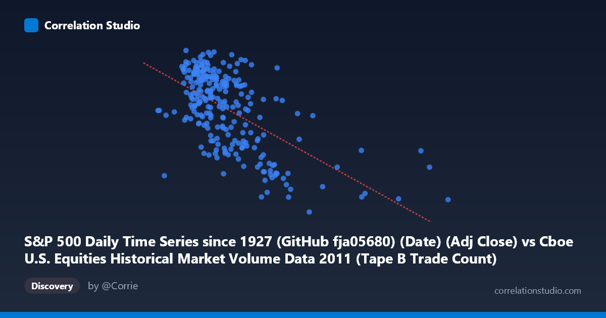
S&P 500 Daily Time Series since 1927 (GitHub fja05680) (Date) (Adj Close) vs Cboe U.S. Equities Historical Market Volume Data 2011 (Tape B Trade Count)

Pearson correlation (r): -0.6091
Spearman correlation: -0.5452
p-value: 0
Sample size (n): 252
95% confidence interval: -0.6814 to -0.5251
Granger causality: None
Granger optimal lag: 1

AI analysis

Analysis: S&P 500 Adjusted Close vs. Cboe Tape B Trade Count (2011)

Relationship Overview The scatterplot reveals a moderate negative relationship between the S&P 500 adjusted closing price and the Cboe Tape B trade count across 2011 trading days. As the S&P 500 price rises, the number of Tape B trades tends to decrease, and vice versa. The linear regression equation (y = −0.000364x + 1,370) captures this downward slope, though the scatter around the regression line is substantial, indicating meaningful variability unexplained by price level alone. The data spans a wide X range (~109K to ~832K in trade count units), though the bulk of observations cluster below 450K, with a sparse tail of higher-volume outliers.

Correlation Strength and Statistical Significance The Pearson correlation of r = −0.6091 indicates a moderate-to-strong negative association, and the R² of 0.371 means that roughly 37% of the variance in Tape B trade counts is explained by the S&P 500 price level — meaningful, but leaving 63% attributable to other factors. The 95% confidence interval of [−0.68, −0.53] is reasonably tight and entirely negative, confirming the direction of the relationship with confidence. The p-value of effectively zero, combined with N = 3,780 and n = 252 paired observations, makes this result highly statistically robust. However, the Granger causality analysis reveals no significant temporal predictive relationship in either direction (X→Y: F = 0.156, p = 0.69; Y→X: F = 0.038, p = 0.85). This is critical: while the two variables are contemporaneously correlated, neither reliably predicts the other's future values at a one-period lag, suggesting the relationship is associative rather than directionally causal at short timescales.

Patterns, Clusters, and Outliers The scatterplot shows a relatively dense central cluster between S&P prices of roughly 175K–375K and Tape B trade counts of 1,150–1,360, consistent with the mean and standard deviation of both variables. There is a visible downward-sloping trend through this core cluster, but with considerable vertical spread — many price levels correspond to a wide range of trade counts, suggesting substantial day-to-day noise. A few notable outliers appear in the upper-right region (higher S&P prices paired with moderate-to-high trade counts) and at very low S&P values with correspondingly high trade counts, which anchor the negative slope. One point near (556K, 1,173) and another near (495K, 1,257) sit at elevated X values with lower Y values, consistent with the negative trend but also potentially representing unusual market sessions.

Confounding Factors and Caveats Several important caveats apply. First, 2011 was a particularly volatile year for U.S. equities, featuring the August debt-ceiling crisis and European sovereign debt fears, which simultaneously depressed prices and triggered elevated trading volumes — this single-year snapshot may overstate a relationship that is largely crisis-driven rather than structural. Second, the X-axis labels reference "Adj Close" values but the data range (109K–832K) is inconsistent with typical S&P 500 price levels (~1,100–1,360 in 2011), suggesting a possible data mapping or axis label issue that warrants verification. Third, Tape B covers NYSE American (AMEX)-listed securities specifically, so its trade count reflects a subset of overall market activity rather than the broad market the S&P 500 represents. Omitted variables — such as VIX levels, macroeconomic news events, or algorithmic trading patterns — likely drive much of the unexplained variance.

Actionable Insights and Further Investigation Given the moderate correlation and absence of Granger causality, practitioners should avoid using S&P 500 price level alone as a predictor of Tape B trading volume in short-term models. Further investigation should include: (1) incorporating market volatility (VIX) as a potential mediating or confounding variable, since fear-driven selloffs affect both price and volume simultaneously; (2) extending the analysis across multiple years to test whether this negative relationship is specific to 2011's crisis environment or is more persistent; (3) examining non-linear models (e.g., quadratic or piecewise regression), as the scatter hints at heteroscedasticity and possible regime-dependent behavior; and (4) resolving the axis label discrepancy to ensure the X-variable truly represents what is described. A VAR (vector autoregression) model incorporating additional market microstructure variables could also shed light on why Granger causality fails despite the contemporaneous correlation.

X dataset: Cboe U.S. Equities Historical Market Volume Data 2011

Y dataset: S&P 500 Daily Time Series since 1927 (GitHub fja05680) (Date)

Part of experiment: Daily - Cboe U.S. Equities Historical Market Volume Data 2011 vs S&P 500 Daily Time Series since 1927 (GitHub fja05680) (Date)