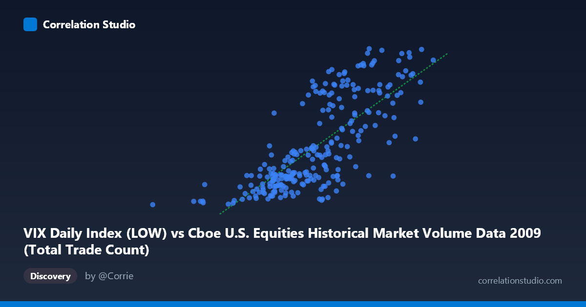
VIX Daily Index (LOW) vs Cboe U.S. Equities Historical Market Volume Data 2009 (Total Trade Count)
- Pearson correlation (r)
- 0.7565
- Spearman correlation
- 0.777
- p-value
- 0
- Sample size (n)
- 252
- 95% confidence interval
- 0.6982 to 0.8048
- Granger causality
- None
- Granger optimal lag
- 1
AI analysis
Analysis: VIX Daily Index (Low) vs. Total Trade Count (2009)
Relationship Overview The scatterplot reveals a moderately strong positive relationship between the VIX Daily Index Low values and the Total Trade Count in U.S. equities markets during 2009. As the VIX Low increases, trade counts tend to rise meaningfully, suggesting that periods of elevated volatility (even at daily lows) coincide with heightened trading activity. This is intuitively consistent with market behavior: fear and uncertainty drive participants to reposition portfolios, hedge exposures, or capitalize on price dislocations, all of which inflate transaction volumes. The linear regression equation (y = 1.09×10⁻⁵x + 1.47) confirms a positive slope, though the relatively small coefficient reflects the scale disparity between the two variables.
Correlation Strength and Statistical Robustness The Pearson correlation of r = 0.7565 indicates a substantial positive association, and the r² of 0.5723 means that approximately 57.2% of the variance in Total Trade Count is explained by the VIX Low — a meaningful but incomplete explanation, leaving ~43% attributable to other factors. The 95% confidence interval of [0.698, 0.805] is reassuringly narrow, and the p-value of effectively zero across a paired sample of 252 observations (drawn from a population of 3,232) confirms this is not a chance finding. However, the Granger causality results are notably inconclusive: neither direction (X→Y: F=0.256, p=0.613; Y→X: F=0.046, p=0.830) achieves significance, meaning that while the two variables move together contemporaneously, neither reliably predicts the other in a lagged temporal sense. This is an important caveat — correlation here does not imply a leading-indicator relationship.
Patterns, Clusters, and Outliers The scatterplot shows several distinct structural features worth noting: - A dense lower-left cluster around VIX Low values of 20–25 and relatively modest trade counts, representing the calmer stretches of 2009 (mid-to-late year as markets stabilized post-crisis) - A dispersed upper-right cluster at VIX Low values of 40–50 with high trade counts, corresponding to the volatile early-2009 period surrounding market lows in February–March - Potential outliers at extreme X values (e.g., the point near X=629,671, Y=19.25 and X=4,134,002, Y=47.08) that may exert disproportionate leverage on the regression line - Some heteroscedasticity appears present — variance in trade counts fans out at higher VIX levels, suggesting the relationship becomes less predictable under high-volatility regimes
Confounding Factors and Caveats Several important confounds complicate a clean causal interpretation. First, 2009 was an extraordinary year — spanning the tail of the global financial crisis and a historic market bottom in March — meaning the data captures an unusually wide volatility regime that may not generalize to normal market conditions. Second, algorithmic and high-frequency trading volumes were surging in this period, and such activity responds to volatility non-linearly, potentially inflating the correlation. Third, the axis labels appear inverted relative to the dataset descriptions (VIX Low is on the X-axis but sourced from the market volume dataset, and trade count is on the Y-axis but sourced from the VIX dataset), which warrants verification of data alignment before drawing firm conclusions. Finally, the absence of Granger causality suggests a common driver — such as macroeconomic shock events — may be simultaneously moving both variables rather than one causing the other.
Actionable Insights and Further Investigation Practitioners should avoid using VIX Low as a standalone leading indicator for trade volume given the failed Granger tests, despite the strong contemporaneous correlation. Instead, both variables likely respond to the same underlying market stress signals. Further investigation should include: (1) regime-segmented analysis separating the crisis period (Q1 2009) from the recovery (Q2–Q4) to test whether the correlation holds across regimes; (2) nonlinear modeling (e.g., log transformation or spline regression) to better capture the heteroscedastic fanning visible at high VIX levels; (3) inclusion of confounders such as S&P 500 realized volatility, Fed intervention dates, or earnings announcement calendars; and (4) extension to multi-year data to assess whether this relationship persists outside the crisis context or is an artifact of 2009's extreme conditions.
X dataset: Cboe U.S. Equities Historical Market Volume Data 2009
Y dataset: VIX Daily Index
Part of experiment: Daily - Cboe U.S. Equities Historical Market Volume Data 2009 vs VIX Daily Index