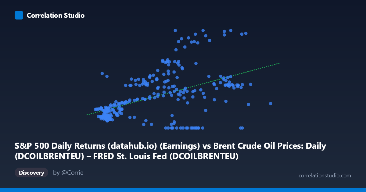
S&P 500 Daily Returns (datahub.io) (Earnings) vs Brent Crude Oil Prices: Daily (DCOILBRENTEU) – FRED St. Louis Fed (DCOILBRENTEU)
- Pearson correlation (r)
- 0.5158
- Spearman correlation
- 0.4874
- p-value
- 0
- Sample size (n)
- 297
- 95% confidence interval
- 0.4271 to 0.5947
- Granger causality
- None
- Granger optimal lag
- 1
AI analysis
S&P 500 Earnings vs. Brent Crude Oil Prices: Correlation Analysis
Overall Relationship The scatterplot reveals a moderate positive relationship between S&P 500 earnings (X-axis) and Brent Crude Oil prices (Y-axis), spanning nearly four decades from 1987 to 2026. The linear regression equation (y = 0.730x + 24.01) suggests that for every unit increase in S&P 500 earnings, Brent crude prices rise by approximately $0.73 per barrel. While this positive trend is visually discernible, the data points exhibit considerable scatter around the regression line, immediately signaling that the relationship is far from deterministic and that other forces are substantially shaping crude oil prices independently of equity earnings.
Correlation Strength and Statistical Significance The Pearson correlation of r = 0.516 indicates a moderate positive association, but the more informative metric is r² = 0.266 — meaning S&P 500 earnings explain only 26.6% of the variance in Brent crude prices, leaving roughly 73.4% attributable to other factors. The 95% confidence interval [0.427, 0.595] is reasonably tight and does not cross zero, and the p-value of effectively 0 across N = 1,865 observations confirms this correlation is statistically robust and not a sampling artifact. However, the Granger causality tests tell a critically important story: neither variable significantly predicts the other in temporal sequence (X→Y: F = 1.40, p = 0.237; Y→X: F = 0.56, p = 0.457). This means the correlation reflects co-movement, likely driven by shared macroeconomic forces, rather than any directional predictive relationship — a crucial caveat for any trading or forecasting application.
Notable Patterns, Clusters, and Outliers Several structural features stand out in the data: - Dense low-value cluster: A large concentration of points at low X values (roughly 10–35) with Y values spanning 0–50 suggests a prolonged period of modest earnings and low oil prices, likely corresponding to pre-2000 and post-2014 regimes - High-dispersion middle range: Points in the X range of 50–90 show dramatically high variance in Y (from near 0 to ~190), indicating that at moderate earnings levels, oil prices behave nearly unpredictably — classic evidence of regime-dependent behavior - Zero-value Y observations: Multiple data points sit at Y = 0 (e.g., coordinates (73.63, 0.00), (67.09, 0.00), (84.82, 0.00), (86.92, 0.00)), which are likely data quality artifacts or missing value substitutions rather than genuine zero oil prices and should be flagged for data cleaning - Extreme high-Y outliers: Points such as (84.51, 190.39), (81.61, 174.36), (83.68, 175.17), and (86.28, 172.75) represent oil price spikes (likely 2008 or 2022 commodity surges) that sit well above the regression line, pulling the fit and inflating variance
Confounding Factors and Interpretive Caveats This correlation is almost certainly spurious co-integration driven by shared macroeconomic growth trends rather than a direct causal mechanism. Both S&P 500 earnings and oil prices rise during global economic expansions and fall during recessions, creating an apparent link that would largely disappear when controlling for GDP growth or industrial output. Additional confounders include: OPEC supply decisions (exogenous to equity markets), USD exchange rate fluctuations (oil is dollar-denominated), geopolitical shocks (Gulf Wars, Russia-Ukraine), and energy sector weighting in the S&P 500 itself, which creates a partial mechanical relationship. The axis labels also warrant scrutiny — the dataset descriptions appear swapped (X is labeled as S&P earnings from a Brent dataset, Y as Brent prices from an S&P dataset), suggesting a metadata alignment issue that should be verified before drawing conclusions.
Actionable Insights and Further Investigation Given these findings, several investigative paths are warranted: 1. Resolve the zero-value anomalies — audit and remove or impute the Y = 0 observations before any modeling work 2. Regime-segmented analysis — split the data into distinct oil market regimes (pre-2000, 2000–2014, post-2014) to test whether the correlation is stable or driven by a specific historical period 3. Control for GDP/industrial production — run a partial correlation removing macroeconomic growth trends to test whether any relationship persists independently 4. Nonlinear modeling — the high variance at moderate X values and outlier clustering suggests a piecewise or threshold regression may capture the relationship far better than the linear model 5. Cross-validate the Granger test with longer lags — the current test used only lag-1; testing lags 3–12 months may reveal delayed transmission mechanisms between earnings cycles and commodity pricing that the current specification misses
X dataset: Brent Crude Oil Prices: Daily (DCOILBRENTEU) – FRED St. Louis Fed
Y dataset: S&P 500 Daily Returns (datahub.io)
Part of experiment: Daily - Brent Crude Oil Prices: Daily (DCOILBRENTEU) – FRED St. Louis Fed vs S&P 500 Daily Returns (datahub.io)