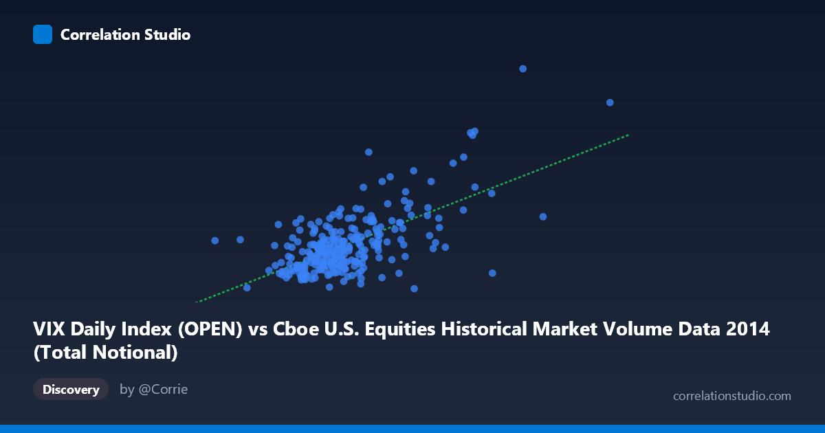
VIX Daily Index (OPEN) vs Cboe U.S. Equities Historical Market Volume Data 2014 (Total Notional)
- Pearson correlation (r)
- 0.6376
- Spearman correlation
- 0.4982
- p-value
- 0
- Sample size (n)
- 252
- 95% confidence interval
- 0.558 to 0.7056
- Granger causality
- None
- Granger optimal lag
- 1
AI analysis
Analysis: VIX Daily Index vs. U.S. Equities Market Volume (2014)
Relationship Overview The scatterplot reveals a positive relationship between the Cboe VIX Daily Index (open) on the X-axis and Total Notional market volume on the Y-axis across 252 trading days in 2014. As market volume increases, VIX levels tend to rise as well, which aligns with well-established financial theory: periods of elevated trading activity are frequently associated with heightened uncertainty and volatility. The linear regression equation (y = 4.37×10⁻¹⁰x + 6.46) confirms this upward slope, though the intercept suggests a baseline VIX level exists independent of volume fluctuations.
Correlation Strength and Statistical Significance The correlation of r = 0.638 indicates a moderate-to-strong positive association, and the r² of 0.407 means that approximately 40.7% of the variance in VIX levels is explained by market volume — a meaningful but incomplete explanation, leaving roughly 59% attributable to other factors. The 95% confidence interval [0.558, 0.706] is relatively narrow and does not include zero, and the p-value is effectively zero, confirming that this relationship is highly statistically significant and unlikely to be a sampling artifact. However, the Granger causality results tell a more cautionary story: neither direction (X→Y nor Y→X) achieves statistical significance (F = 0.677, p = 0.411 and F = 0.039, p = 0.845, respectively). This means that while the two variables are correlated contemporaneously, neither reliably predicts the other's future values at a one-period lag, undermining any simple causal narrative.
Notable Patterns, Clusters, and Outliers The sample points reveal several notable features. The bulk of observations cluster in the volume range of roughly 13–22 billion with VIX values between 11 and 17, suggesting a relatively stable "normal" regime for 2014. However, there are clear high-leverage outliers: the point at approximately (31.2B, 29.26) stands conspicuously apart and likely corresponds to a specific volatility spike event (potentially the October 2014 market selloff). Similarly, the point near (27.3B, 23.55) reinforces the pattern that extreme volume days correspond to elevated VIX. Conversely, the point at (22.9B, 10.40) represents an interesting counter-example — very high volume with low VIX — suggesting that not all high-volume days are fear-driven. The minimum X value point (7.69B, 14.52) also warrants attention as an outlier on the low-volume end with a moderate VIX reading.
Confounding Factors and Caveats Several important caveats apply to this interpretation. First, reverse causality and simultaneity are plausible: high VIX may prompt institutional hedging activity that itself drives volume, rather than volume causing volatility. Second, seasonal effects in 2014 (e.g., summer doldrums, year-end positioning) could simultaneously suppress both metrics or inflate them, creating spurious correlation. Third, the dataset covers only a single calendar year (2014), limiting generalizability; 2014 included specific macro events (geopolitical tensions, Fed tapering completion, Ebola fears) that may have created an unusually strong volume-volatility coupling not representative of other periods. Finally, the axes are swapped from the intuitive convention (VIX as X, volume as Y), which may affect interpretive framing, and the dataset-column label assignments suggest possible metadata misalignment that should be verified.
Actionable Insights and Further Investigation Practitioners should avoid using contemporaneous volume as a standalone VIX predictor given the Granger causality failure — the relationship does not hold predictive power at even a one-period lag. Instead, this correlation is better understood as a coincident indicator: both variables respond to the same underlying market stress events simultaneously. Further investigation should include: (1) extending the analysis across multiple years to test whether the r ≈ 0.64 relationship is stable or regime-dependent; (2) examining intraday data to better resolve lead-lag dynamics that daily aggregation may obscure; (3) controlling for known confounders such as options expiration dates, macroeconomic announcements, and Federal Reserve meeting days; and (4) applying non-linear models (e.g., threshold regression or regime-switching models) given the apparent clustering and the presence of outliers that disproportionately drive the linear fit.
X dataset: Cboe U.S. Equities Historical Market Volume Data 2014
Y dataset: VIX Daily Index
Part of experiment: Daily - Cboe U.S. Equities Historical Market Volume Data 2014 vs VIX Daily Index