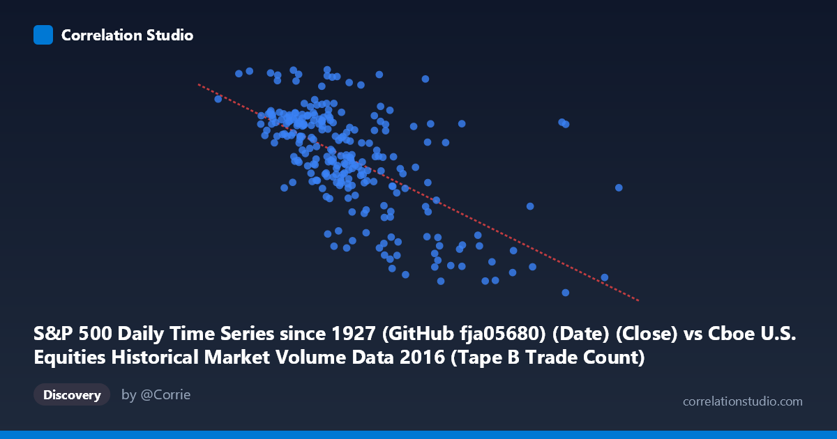
S&P 500 Daily Time Series since 1927 (GitHub fja05680) (Date) (Close) vs Cboe U.S. Equities Historical Market Volume Data 2016 (Tape B Trade Count)

Pearson correlation (r): -0.6209
Spearman correlation: -0.6203
p-value: 0
Sample size (n): 252
95% confidence interval: -0.6914 to -0.5386
Granger causality: None
Granger optimal lag: 1

AI analysis

Analysis: S&P 500 Close Price vs. Cboe Tape B Trade Count (2016)

1. Overall Relationship The scatterplot reveals a moderate negative relationship between the S&P 500 daily closing price and Cboe Tape B trade count throughout 2016. As the S&P 500 close price increases (moving right along the x-axis), the Tape B trade count tends to decrease, following the linear regression equation y = −0.000664x + 2306.67. This inverse pattern suggests that on days when equity prices were higher, the volume of smaller-cap or regional exchange trades (Tape B securities) was generally lower — an intuitively plausible dynamic if rising markets correlate with reduced panic-driven or speculative trading activity in mid-tier listings.

2. Correlation Strength, Direction, and Causality The Pearson correlation of r = −0.621 indicates a moderate-to-strong negative association, and the R² of 0.385 means that roughly 38.5% of the variance in Tape B trade counts is statistically explained by the S&P 500 close price level. While meaningful, this also implies that 61.5% of the variance remains unexplained, pointing to substantial additional drivers. The 95% confidence interval of [−0.691, −0.539] is relatively tight and does not cross zero, and the p-value is effectively 0 (with N = 3,622), confirming the correlation is highly statistically significant and not a sampling artifact. However, the Granger causality results are notably absent in both directions — neither X→Y (F = 0.346, p = 0.557) nor Y→X (F = 0.181, p = 0.671) reaches significance — meaning there is no detectable temporal predictive relationship at a one-period lag. This is a critical caveat: the correlation reflects a contemporaneous co-movement, not a leading/lagging signal that could be exploited for prediction.

3. Notable Patterns, Clusters, and Outliers The data cloud shows a broadly linear downward trend but with considerable scatter, particularly in the mid-range of X (roughly 250,000–380,000). Several notable features stand out: - A cluster of high trade counts (Y 2,150) is concentrated at lower price levels (X < 300,000), consistent with elevated trading activity during early-2016 market volatility - Outliers at high X values (e.g., points near 558,190 and 467,365 with Y around 1,868–1,883) sit well to the right of the main cluster, likely representing specific high-volume price days that anchor the regression slope - One point near (362,471; 2,262) appears as an upward outlier — high trade count despite a moderate price level — which warrants individual investigation - The upper-left quadrant (low price, high trade count) is densely populated, reinforcing the inverse trend, while the lower-right quadrant contains sparser but influential high-leverage points

4. Confounding Factors and Interpretive Caveats Several important confounds complicate a causal interpretation. First, both variables are time-indexed to 2016, meaning secular trends — the market's gradual recovery and rally during 2016 — could drive the negative correlation spuriously; rising prices over the year naturally coincide with changing market microstructure and participation patterns. Second, Tape B specifically covers NYSE American (AMEX) and regional exchange-listed securities, which may respond differently to macro conditions than the broader S&P 500 constituents. Third, major discrete events in 2016 (Brexit in June, the U.S. election in November) likely generated structural breaks in the data that the linear model smooths over. Finally, the absence of Granger causality at lag-1 suggests the relationship is contemporaneous and possibly driven by a common underlying factor (e.g., market volatility, institutional sentiment) rather than either variable mechanistically influencing the other.

5. Actionable Insights and Further Investigation Practitioners should avoid treating this correlation as a predictive signal — the Granger non-causality result explicitly rules out using one variable to forecast the other at a one-period lag. Instead, several follow-up analyses are warranted: (a) decompose the time series to separate trend from cyclical components and test whether the correlation persists after detrending, which would isolate true co-movement from shared drift; (b) incorporate VIX or realized volatility as a covariate, as volatility likely explains a substantial portion of the residual 61.5% variance and may mediate the observed relationship; (c) test multiple Granger lags beyond lag-1, given that market microstructure effects can manifest over days or weeks; and (d) segment the analysis by market regime (pre/post-Brexit, pre/post-election) to assess whether the correlation coefficient is stable or driven by specific high-volatility episodes. The outlier cluster at high X values should also be examined for data quality or event-specific explanations before drawing broader conclusions.

X dataset: Cboe U.S. Equities Historical Market Volume Data 2016

Y dataset: S&P 500 Daily Time Series since 1927 (GitHub fja05680) (Date)

Part of experiment: Daily - Cboe U.S. Equities Historical Market Volume Data 2016 vs S&P 500 Daily Time Series since 1927 (GitHub fja05680) (Date)