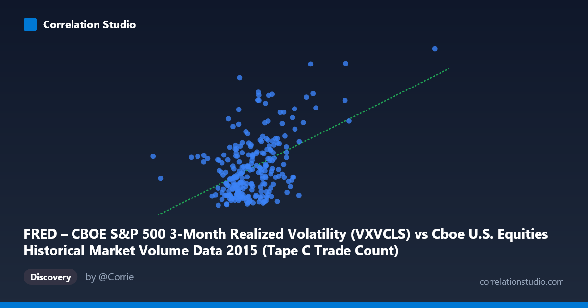
FRED – CBOE S&P 500 3-Month Realized Volatility (VXVCLS) vs Cboe U.S. Equities Historical Market Volume Data 2015 (Tape C Trade Count)
- Pearson correlation (r)
- 0.4699
- Spearman correlation
- 0.3483
- p-value
- 0
- Sample size (n)
- 252
- 95% confidence interval
- 0.3677 to 0.5609
- Granger causality
- None
- Granger optimal lag
- 1
AI analysis
Scatterplot Analysis: CBOE S&P 500 3-Month Realized Volatility vs. Tape C Trade Count (2015)
Relationship Overview
The scatterplot reveals a moderate positive relationship between CBOE S&P 500 3-month realized volatility (X-axis) and Tape C trade count (Y-axis) across 252 trading days in 2015. The linear regression equation (y = 1.14256E-05x + 9.85009) confirms that as market volume/notional activity increases, realized volatility tends to rise alongside it. This is conceptually intuitive — elevated trading activity in U.S. equities markets is often associated with periods of heightened uncertainty or price discovery, which would naturally manifest in higher realized volatility readings. The relationship is visible but noisy, with considerable scatter around the regression line, suggesting the association is real but far from deterministic.
Correlation Strength and Statistical Significance
The Pearson correlation of r = 0.4699 indicates a moderate positive association, but the explanatory power is meaningfully limited: r² = 0.2208 means only ~22.1% of the variance in volatility is explained by Tape C trade count, leaving roughly 78% attributable to other factors. The 95% confidence interval of [0.3677, 0.5609] is reasonably tight and does not approach zero, lending confidence that the true population correlation is genuinely positive. The p-value of 3.109E-15 is extraordinarily small, effectively ruling out chance as an explanation given the sample size of 252 (drawn from a population of 3,302). However, it is critical to note that Granger causality tests find no significant predictive directionality in either direction — neither X→Y (F = 0.0917, p = 0.7623) nor Y→X (F = 0.2715, p = 0.6028) — meaning that past values of trade count do not help forecast future volatility and vice versa at a 1-period lag. The relationship is contemporaneous in nature, not temporally predictive.
Notable Patterns, Clusters, and Outliers
Several features stand out in the sample points. The bulk of observations cluster between roughly 600,000–900,000 on the X-axis and 14–22 on the Y-axis, forming a dense core that anchors the regression. However, there are notable high-leverage outliers in both dimensions: the point at approximately (1,194,527, 29.58) and (1,210,005, 23.47) sit far to the right and above the main cluster, likely corresponding to the August 2015 market volatility episode — a period of sharp equity selloff and extreme volume spikes. Conversely, the point at (291,078, 19.69) is an extreme low-volume outlier on the X-axis, potentially reflecting a holiday-shortened trading session. There also appears to be a heteroscedastic pattern — variance in Y widens at higher X values — suggesting the linear model may underfit the high-volatility regime. A handful of high-Y, moderate-X points (e.g., ~696,002, 28.07) suggest volatility can spike independently of volume surges.
Confounding Factors and Caveats
Several important caveats apply. First, Tape C specifically captures NYSE Arca-listed securities, meaning this trade count may not fully represent broad market activity — cross-market dynamics, dark pool volumes, or exchange routing shifts could distort the signal. Second, realized volatility is a backward-looking 3-month measure, which inherently smooths over daily volume spikes and creates a temporal mismatch with daily trade counts; this lag structure likely suppresses both the correlation magnitude and the Granger causality signal. Third, 2015 is a single calendar year with a specific macro regime (China slowdown fears, Fed tightening expectations, the August flash crash), making generalizability to other periods uncertain. Fourth, the relationship could be spuriously driven by a common cause — market stress events simultaneously drive both volume and volatility, meaning the correlation may reflect shared responses to external shocks rather than any direct mechanism between the two variables.
Actionable Insights and Further Investigation
Given the moderate correlation and absence of Granger causality, practitioners should be cautious about using Tape C trade counts as a leading indicator of volatility for trading or risk management purposes. However, the contemporaneous relationship does suggest that real-time volume monitoring could serve as a coincident signal of elevated volatility regimes rather than a predictive one. Further investigation should include: (1) testing across multiple years to assess whether the 2015 relationship is regime-specific or persistent; (2) incorporating implied volatility (VIX) alongside realized volatility to disentangle forward-looking versus backward-looking dynamics; (3) applying a non-linear model or regime-switching framework to better capture the apparent heteroscedasticity at high-volume extremes; and (4) testing at different Granger lags (beyond 1 period) to determine if a longer memory structure exists between these variables.
X dataset: Cboe U.S. Equities Historical Market Volume Data 2015
Y dataset: FRED – CBOE S&P 500 3-Month Realized Volatility
Part of experiment: Daily - Cboe U.S. Equities Historical Market Volume Data 2015 vs FRED – CBOE S&P 500 3-Month Realized Volatility