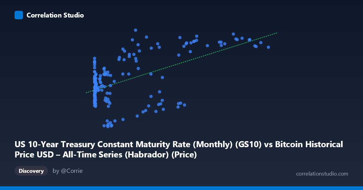
US 10-Year Treasury Constant Maturity Rate (Monthly) (GS10) vs Bitcoin Historical Price USD – All-Time Series (Habrador) (Price)
- Pearson correlation (r)
- 0.5848
- Spearman correlation
- 0.3595
- p-value
- 0
- Sample size (n)
- 189
- 95% confidence interval
- 0.4823 to 0.6715
- Granger causality
- None
- Granger optimal lag
- 1
- Time coverage
- 2010-08-01 to 2026-04-01
- Recomputed on refreshed data
- 2026-10-08 (r was 0.5848)
AI analysis
Analysis: Bitcoin Price vs. US 10-Year Treasury Rate
1. What the Visualization Reveals
The scatterplot shows a positive but noisy relationship between Bitcoin price (X-axis, ranging from $0.06 to $118,670) and the US 10-Year Treasury Constant Maturity Rate (Y-axis, ranging from 0.62% to 4.80%). At low Bitcoin prices (under $1,000), Treasury yields cluster tightly in the 1.6–3.0% range, reflecting the low-rate environment of the early-to-mid 2010s. As Bitcoin's price climbs into the tens of thousands of dollars, the yield values spread out and trend higher, with several points clustering near 4.0–4.6% at the highest Bitcoin prices (e.g., $85K–$118K range). This pattern suggests the relationship is driven largely by both series moving together over calendar time, rather than a direct causal link between them.
2. Strength, Direction, and Uncertainty
The correlation coefficient (r = 0.585) indicates a moderate positive relationship, with r² = 0.342 meaning only about 34% of the variance in Treasury yields is statistically explained by Bitcoin price (or vice versa) — leaving nearly two-thirds unexplained. The 95% confidence interval [0.48, 0.67] is reasonably tight and excludes zero, and the p-value of ~0 confirms this correlation is highly unlikely to be due to chance given the sample size (n=189). However, statistical significance should not be conflated with practical predictive power — r² of 0.34 is modest. Critically, the Granger causality tests show no significant predictive direction in either direction (Bitcoin→Yield: p=0.93; Yield→Bitcoin: p=0.25). This strongly suggests the correlation is not driven by one variable temporally leading the other, but more likely reflects a shared underlying trend (e.g., both rising over the 2010–2026 macro cycle) rather than genuine cause-and-effect dynamics.
3. Notable Patterns and Outliers
A key non-linear feature is the heteroskedasticity: variance in Y increases substantially as X grows. Low Bitcoin prices show compressed yield values (mostly 1.6–3.0%), while high Bitcoin prices show much wider dispersion (1.3% to 4.8%), including notable outliers like ($58,724, 1.64%), ($41,870, 1.28%), and ($34,856, 1.32%) — cases where Bitcoin was elevated but yields were unusually low, likely corresponding to the 2020–2021 near-zero-rate, high-BTC-price era. Conversely, points like ($27,984, 4.80%) and ($94,757, 4.63%) show high yields coinciding with high-to-moderate BTC prices, likely reflecting 2023–2024 rate-hiking cycles. This scatter pattern looks more like two independent trending time series overlaid than a tight causal relationship, consistent with the null Granger result.
4. Confounding Factors and Caveats
The most important caveat is that time is the dominant confound. Both Bitcoin price and Treasury yields have exhibited strong secular trends over 2010–2026 (Bitcoin's multi-year appreciation from fractions of a cent to six figures; Treasury yields cycling from near-zero post-2008/2020 to elevated post-2022 levels). Any two trending time series will show spurious correlation even absent a causal mechanism. Additionally, this is monthly data spanning 15+ years, so structural breaks (2013, 2017, 2020-21, 2022 hiking cycle) mean the relationship is unlikely to be stationary or consistent across the full period. The linear regression (slope ≈ 1.99e-5) is also heavily influenced by the extreme skew in Bitcoin's price distribution (mean $20,533, stdev $29,894), where a handful of very high-price observations exert outsized leverage.
5. Suggestions for Further Investigation
Given the lack of Granger causality, treat this correlation as descriptive rather than predictive. Recommended next steps: (a) detrend or difference both series (e.g., analyze month-over-month returns/changes rather than levels) to test whether short-term co-movements exist once long-term trends are removed; (b) segment the analysis by macro regime (pre-2020 vs. post-2020) to check for regime-dependent relationships, since the near-zero-rate 2020-21 period likely drives much of the apparent correlation; (c) consider log-transforming Bitcoin price given its extreme right-skew, which may better linearize the relationship; and (d) incorporate a third variable (e.g., broad risk appetite, DXY, or M2 money supply) as a potential common driver behind both series' trends, since Treasury yields and Bitcoin may both simply be responding to macro liquidity conditions rather than to each other.
X dataset: Bitcoin Historical Price USD – All-Time Series (Habrador)
Y dataset: US 10-Year Treasury Constant Maturity Rate (Monthly)
Part of experiment: Bitcoin - Bitcoin Historical Price USD – All-Time Series (Habrador) vs US 10-Year Treasury Constant Maturity Rate (Monthly)