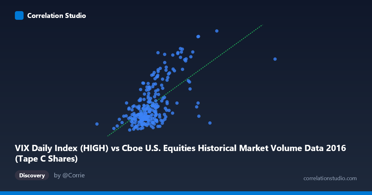
VIX Daily Index (HIGH) vs Cboe U.S. Equities Historical Market Volume Data 2016 (Tape C Shares)
- Pearson correlation (r)
- 0.6241
- Spearman correlation
- 0.5468
- p-value
- 0
- Sample size (n)
- 252
- 95% confidence interval
- 0.5423 to 0.6941
- Granger causality
- None
- Granger optimal lag
- 1
AI analysis
Scatterplot Analysis: VIX High vs. Tape C Shares (2016)
Relationship Overview The scatterplot reveals a moderate positive relationship between the CBOE VIX Daily High Index and Tape C share volume in U.S. equities markets during 2016. As VIX readings rise — indicating higher expected market volatility — Tape C trading share volumes tend to increase as well. This is intuitively consistent with market microstructure theory: elevated fear or uncertainty typically drives heightened trading activity as investors rebalance, hedge, or liquidate positions. The linear regression equation (y = 1.009×10⁻⁷x + 3.44) confirms a positive slope, though the relatively small coefficient reflects the vast scale difference between the two variables.
Correlation Strength and Statistical Significance The Pearson correlation of r = 0.6241 indicates a moderate-to-strong positive association, and with a p-value of essentially zero and a tight 95% confidence interval of [0.5423, 0.6941], this result is highly statistically robust across the 252-day paired sample drawn from a population of 3,622 observations. However, r² = 0.3895 is the more sobering figure — it means that only ~39% of the variance in Tape C volume is explained by VIX High levels alone, leaving roughly 61% attributable to other factors entirely. Critically, the Granger causality tests reveal no significant temporal predictive relationship in either direction (X→Y: F = 0.138, p = 0.711; Y→X: F = 0.151, p = 0.698). This means that while the two variables move together contemporaneously, neither reliably predicts the other in advance at a 1-period lag, which substantially limits any causal or forecasting interpretation.
Notable Patterns, Clusters, and Outliers The sample points reveal meaningful structural features. The bulk of observations cluster in a lower-left band — VIX readings roughly between 11–18 paired with moderate share volumes — suggesting that "normal" 2016 market conditions dominated the year. However, several conspicuous outliers pull toward the upper right: points such as (175M, 28.43) and (166M, 23.81) represent high-volatility, high-volume sessions likely tied to discrete macro events (e.g., Brexit, the U.S. presidential election). A secondary cluster at lower VIX values (12–14) with surprisingly variable volume suggests that volume can remain elevated even in calm periods, potentially driven by algorithmic or passive rebalancing activity independent of fear. This heteroscedastic spread — variance in Y increasing with X — is a notable non-linear feature that a simple linear model may underfit.
Confounding Factors and Caveats Several important caveats temper this analysis. First, Tape C specifically captures NYSE Arca-listed securities, so the relationship may reflect sector-specific dynamics (e.g., ETF trading, tech stocks) rather than broad market behavior. Second, 2016 was an unusual year with identifiable volatility spikes from Brexit (June) and the U.S. election (November), meaning the correlation may be partly event-driven and non-generalizable to other years. Third, the absence of Granger causality at a 1-period lag suggests the relationship is contemporaneous rather than predictive, possibly because both variables respond simultaneously to the same underlying news or macro shocks — a classic case of common-cause confounding. Day-of-week effects, options expiration cycles, and Federal Reserve announcement calendars are additional structural confounders not accounted for here.
Actionable Insights and Further Investigation Despite the causal ambiguity, the moderate correlation offers practical value. Traders and risk managers could use VIX High levels as a same-day signal for expected liquidity conditions in Tape C markets, informing execution timing or transaction cost models. To deepen this analysis, several extensions are warranted: (1) testing Granger causality at longer lags (2–5 periods) to detect slower transmission mechanisms; (2) segmenting the data around identified volatility events to determine whether the correlation is structurally stable or event-dependent; (3) incorporating additional predictors such as options volume, bid-ask spreads, or ETF flow data to build a more complete variance decomposition; and (4) applying a non-linear or quantile regression framework to better capture the apparent heteroscedasticity and tail behavior visible in the high-VIX cluster.
X dataset: Cboe U.S. Equities Historical Market Volume Data 2016
Y dataset: VIX Daily Index
Part of experiment: Daily - Cboe U.S. Equities Historical Market Volume Data 2016 vs VIX Daily Index