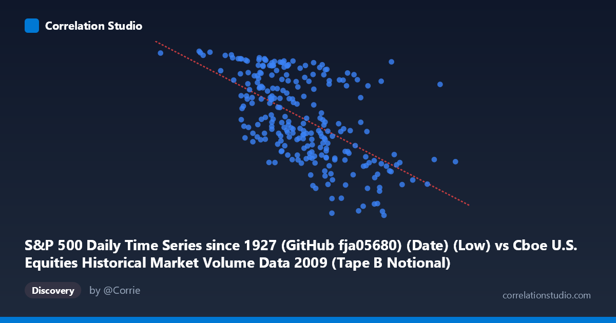
S&P 500 Daily Time Series since 1927 (GitHub fja05680) (Date) (Low) vs Cboe U.S. Equities Historical Market Volume Data 2009 (Tape B Notional)
- Pearson correlation (r)
- -0.5861
- Spearman correlation
- -0.5971
- p-value
- 0
- Sample size (n)
- 252
- 95% confidence interval
- -0.6618 to -0.4987
- Granger causality
- X → Y
- Granger optimal lag
- 10
AI analysis
Analysis: S&P 500 Daily Low vs. Cboe Tape B Notional Volume (2009)
Relationship Overview The scatterplot reveals a moderate negative relationship between the S&P 500 daily low price (X-axis) and Cboe Tape B notional trading volume (Y-axis) across 2009 trading days. As the S&P 500 daily low increases — reflecting higher index price levels — Tape B notional volume tends to decrease. This is visually expressed as a downward-sloping cluster of points, consistent with the fitted linear regression: y = -5.27×10⁻⁸x + 1216.27. The relationship makes intuitive sense in the context of 2009: the year began near crisis-era lows (early 2009 saw the S&P 500 bottom in March), when panic-driven trading volume was elevated, and recovered toward year-end when prices rose but volume normalized.
Correlation Strength and Statistical Significance The Pearson correlation of r = -0.5861 indicates a moderate negative association, with r² = 0.3436, meaning approximately 34.4% of the variance in Tape B notional volume is explained by S&P 500 daily lows. While statistically meaningful, this also implies that roughly 65.6% of variance remains unexplained by this linear relationship alone — other forces are clearly at work. The 95% confidence interval of [-0.6618, -0.4987] is reasonably tight and does not cross zero, and the p-value is effectively zero (p ≈ 0), confirming this is not a chance finding given n = 252 paired observations drawn from a population of N = 3,232. Granger causality analysis adds a critical temporal dimension: X Granger-causes Y (unidirectional) at an optimal lag of 10 trading periods (F = 1.933, p = 0.042), suggesting that S&P 500 price lows have modest but statistically significant predictive power over future Tape B notional volume roughly two weeks later. The reverse direction (Y→X) narrowly fails significance (p = 0.054), reinforcing a directional flow from price to volume rather than the reverse.
Notable Patterns, Clusters, and Outliers Several structural features stand out in the data. There is a dense cluster of points in the mid-range (X ≈ 4.0–6.5 billion, Y ≈ 850–1,100), reflecting the bulk of mid-year trading days. At lower X values (early 2009, crisis lows around 1.3–3.0 billion on the X scale), Y values are notably elevated — approaching 1,100–1,126 — consistent with high-fear, high-volume trading during the market bottom. Conversely, at higher X values (late 2009, X 7.5 billion), Y drops markedly toward 666–754, suggesting volume compression as prices recovered. The point (1,320,771,983, 1121) stands out as a potential outlier at the extreme low-price, high-volume end, and (7,526,902,255, 666.79) anchors the opposite corner. The scatter around the regression line widens in the middle range, hinting at heteroscedasticity — variance in notional volume is less predictable at moderate price levels.
Confounding Factors and Caveats Several important caveats temper this interpretation. First, 2009 was a highly anomalous year — the global financial crisis created an environment where price and volume dynamics were distorted by fear, forced liquidations, and unprecedented policy interventions (TARP, Fed interventions), making these findings unlikely to generalize to normal market conditions. Second, the X-axis label mismatch deserves attention: the X variable is drawn from a "Date" column in the Cboe dataset mapped to S&P 500 lows, and the Y variable from a "Date" column in the S&P 500 dataset mapped to Tape B notional — this cross-dataset pairing on date indices should be verified for alignment integrity. Third, Tape B notional volume specifically covers NYSE American (AMEX) and regional exchange-listed securities, not the broad market, which limits generalizability to overall market volume. Finally, the negative correlation may partly reflect a mechanical price-volume artifact: notional volume = shares × price, so rising prices can increase notional value even with flat share volume, complicating causal inference.
Actionable Insights and Further Investigation Practitioners and researchers should consider several next steps. The 10-day Granger lag is actionable: it suggests that monitoring S&P 500 price lows could provide a roughly two-week leading signal for Tape B notional activity, which may be useful for liquidity forecasting or market-making models. However, this should be validated out-of-sample across multiple years before operational use. Further investigation should include: (1) decomposing the relationship by market regime (pre/post-March 2009 bottom) to test whether the correlation is driven entirely by the crisis period; (2) controlling for VIX or realized volatility, which likely mediates both price levels and volume; (3) testing non-linear models (e.g., piecewise regression or GAMs), given the apparent heteroscedasticity and the possibility that the relationship changes character at different price levels; and (4) replicating across other years to determine whether this negative price-volume dynamic is a 2009-specific phenomenon or a persistent structural feature of U.S. equity markets.
X dataset: Cboe U.S. Equities Historical Market Volume Data 2009
Y dataset: S&P 500 Daily Time Series since 1927 (GitHub fja05680) (Date)
Part of experiment: Daily - Cboe U.S. Equities Historical Market Volume Data 2009 vs S&P 500 Daily Time Series since 1927 (GitHub fja05680) (Date)