Bitcoin Historical Data (2010-2024) (AdrBalCnt) vs CryptoDataDownload – Binance BTC/USDT Daily OHLCV (High)
- Pearson correlation (r)
- 0.8282
- Spearman correlation
- 0.8972
- p-value
- 0
- Sample size (n)
- 3191
- 95% confidence interval
- 0.8169 to 0.8388
- Granger causality
- Y → X
- Granger optimal lag
- 10
AI analysis
Analysis: Bitcoin Active Address Count vs. Price (High)
1. What the Visualization Reveals
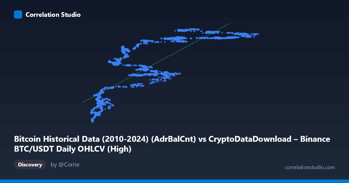
The scatterplot shows a strong positive, monotonic relationship between the number of active Bitcoin addresses (X) and the daily high price (Y). As active address counts increase from roughly 3,000-4,000 up through 100,000+, price highs climb from the low $19-20M range to $50-57M range (values appear scaled, likely representing satoshis or an indexed price unit). The relationship is not perfectly linear—there's a visible steepening and clustering pattern, particularly in the mid-to-upper X range (60,000-90,000), where Y values plateau around $51-57M across a wide span of X, suggesting diminishing marginal price sensitivity to address growth at higher activity levels.
2. Strength, Direction, and Statistical Confidence
With r = 0.828 and R² = 0.686, active address count explains approximately 69% of the variance in price highs—a strong relationship by typical standards, though it leaves nearly a third of price variation unaccounted for by this variable alone. The 95% CI [0.817, 0.839] is tight, and the p-value of ~0 confirms this correlation is highly statistically significant and not a product of sampling noise, especially given the large sample (n=3,191).
However, the Granger causality results complicate a naive "more addresses drive price" narrative: the test indicates Y Granger-causes X (F=1.899, p=0.041), not the reverse (X→Y F=1.459, p=0.149, not significant). This suggests that price movements precede/predict changes in active address counts, not vice versa—consistent with the idea that price rallies attract new wallet activity and speculative entrants, rather than organic adoption growth driving price. This is an important reframing: the correlation is real, but the temporal dynamics point to price as the leading indicator.
3. Notable Patterns and Outliers
Several features stand out: - Low-end cluster: Points with X < 15,000 tightly cluster with Y between $19-33M, showing strong linearity in this region. - Mid-range dispersion: Around X = 20,000-60,000, Y shows more scatter (e.g., X≈24,790 → Y≈33.3M sits well below the trend line formed by nearby points like X≈27,130 → Y≈48.8M), indicating other factors are strongly at play in this zone. - High-end plateau: For X 60,000, Y values compress into a narrow band ($51-57M) despite X ranging widely up to 126,000, suggesting a saturation effect or ceiling in price highs relative to address growth. - This nonlinear "flattening" at high X values hints that a logarithmic or power-law fit might outperform the linear model shown.
4. Confounding Factors and Caveats
Several caveats apply: - Temporal confounding: Both variables likely trend upward over 2017-2026 due to Bitcoin's overall market maturation, meaning shared time-trend (rather than direct causal linkage) could inflate the correlation—classic spurious correlation risk with two non-stationary time series. - Market cycles: Bitcoin's boom-bust cycles (2017, 2021, potential 2024-25 cycles) mean address counts and price may correlate strongly within cycles but diverge across cycles (e.g., post-crash periods with high addresses but low price, or vice versa). - Lag structure: The Granger test's 10-period optimal lag suggests delayed effects are important; a simple contemporaneous scatterplot/correlation may mask the true lead-lag dynamic. - Address count limitations: Active address counts can be inflated by exchange consolidation activity, mixing services, or dust transactions, which don't necessarily reflect genuine network adoption.
5. Actionable Insights
- Test for stationarity and cointegration: Given the Granger result and likely shared trends, run Augmented Dickey-Fuller tests and a cointegration analysis (e.g., Johansen test) to distinguish genuine long-run equilibrium relationships from spurious trend correlation. - Explore nonlinear models: Given the plateau at high X, fit log-linear or spline regressions to better capture the saturation behavior and improve R² beyond 0.686. - Lag-based regression: Since price leads address count, build a predictive model using lagged Y (price) to forecast future X (address activity), which may have more practical value for on-chain analytics than the reverse. - Segment by market regime: Analyze the relationship separately during bull vs. bear markets to see if the r=0.83 correlation holds uniformly or is regime-dependent.
X dataset: CryptoDataDownload – Binance BTC/USDT Daily OHLCV
Y dataset: Bitcoin Historical Data (2010-2024)
Part of experiment: Bitcoin - CryptoDataDownload – Binance BTC/USDT Daily OHLCV vs Bitcoin Historical Data (2010-2024)