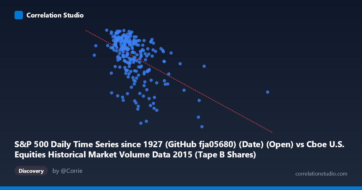
S&P 500 Daily Time Series since 1927 (GitHub fja05680) (Date) (Open) vs Cboe U.S. Equities Historical Market Volume Data 2015 (Tape B Shares)
- Pearson correlation (r)
- -0.4964
- Spearman correlation
- -0.5027
- p-value
- 0
- Sample size (n)
- 252
- 95% confidence interval
- -0.5842 to -0.3972
- Granger causality
- X → Y
- Granger optimal lag
- 7
AI analysis
Analysis: S&P 500 Open Price vs. Cboe Tape B Share Volume (2015)
Relationship Overview The scatterplot reveals a moderate negative relationship between the S&P 500 daily open price (X-axis) and Cboe Tape B share volume (Y-axis) across 252 trading days in 2015. As the S&P 500 open price increases, Tape B share volume tends to decrease. The linear regression equation (y = -9.457×10⁻⁷x + 2159.07) confirms this inverse slope, meaning that for every 10-million-unit increase in the open price index value, Tape B volume declines by roughly 9.5 units. This pattern is broadly consistent with a well-known market dynamic: as equity prices rise during bull-market conditions, share volumes can contract because fewer shares are needed to transact equivalent notional value, and investor complacency may reduce turnover.
Correlation Strength and Statistical Significance The Pearson correlation of r = -0.4964 indicates a moderate negative association, and the R² of 0.2464 means that roughly 24.6% of the variance in Tape B volume is explained by the S&P 500 open price level alone — a meaningful but far from dominant share, leaving ~75% of volume variation unexplained by this single predictor. The 95% confidence interval of [-0.584, -0.397] is entirely negative and does not cross zero, providing strong evidence that the true population correlation is genuinely inverse. The p-value of effectively 0 (across N = 3,302 population observations) confirms this is not a chance finding. Critically, Granger causality runs unidirectionally from X→Y (F = 2.15, p = 0.040) with an optimal lag of 7 trading days, suggesting that S&P 500 open price levels carry statistically meaningful predictive information about Tape B volume approximately one to one-and-a-half weeks later — while the reverse direction (Y→X, p = 0.753) shows no predictive power, reinforcing that volume is the downstream variable here.
Notable Patterns, Clusters, and Outliers The data exhibit a notable fan or wedge structure: at lower S&P 500 open values (roughly 60–90 million range), Tape B volume is highly dispersed, spanning from approximately 1,940 to 2,130, whereas at higher open values (130–215 million), the distribution tightens and clusters at lower volume levels. Several downward outliers are visible — points near (111M, 1920), (128M, 1948), (130M, 1929), and (205M, 1898) — which likely correspond to specific high-volatility or low-liquidity sessions. A loose cluster of high-volume, lower-price observations in the 60–80M range (several points near 2,120–2,130) suggests there may have been a distinct market regime or period of elevated activity early in 2015. The heteroscedasticity in the left portion of the chart hints that a purely linear model may not fully capture the relationship.
Confounding Factors and Caveats Several important caveats apply. First, the X-axis values labeled as "Date (Open)" appear to be encoded as Unix-style timestamps or large numeric date representations rather than intuitive price levels — the range of 44M–312M does not correspond to conventional S&P 500 price points, which suggests a possible data join artifact or column mislabeling that warrants verification before drawing firm conclusions. Second, Tape B specifically covers NYSE American and regional exchange listings, so its volume dynamics may reflect sector-specific or exchange-specific factors unrelated to broad index-level pricing. Third, 2015 was not a uniform year — it included the August 2015 flash crash and periods of heightened volatility, which could produce spurious correlation between price levels and volume if both are jointly driven by episodic risk-off events. Finally, the correlation likely captures a shared time trend (prices generally higher mid-year, volumes fluctuating) rather than a pure causal mechanism.
Actionable Insights and Further Investigation Given the Granger causality finding, practitioners could explore whether a 7-day lagged S&P 500 open price improves short-term Tape B volume forecasting models, potentially useful for exchange capacity planning or algorithmic trading strategies. It would be valuable to decompose the data by market regime (pre/post August 2015 volatility spike) to test whether the correlation holds across sub-periods or is driven by a single episode. Researchers should verify the X-axis encoding — if these are timestamp integers, the axis should be re-expressed as actual calendar dates or price levels to produce a more interpretable and actionable regression coefficient. Finally, incorporating additional predictors — VIX levels, total market notional volume, and Tape A/C volumes — into a multivariate model would help isolate the unique contribution of index price levels to Tape B activity and likely push the explained variance well beyond the current 24.6%.
X dataset: Cboe U.S. Equities Historical Market Volume Data 2015
Y dataset: S&P 500 Daily Time Series since 1927 (GitHub fja05680) (Date)
Part of experiment: Daily - Cboe U.S. Equities Historical Market Volume Data 2015 vs S&P 500 Daily Time Series since 1927 (GitHub fja05680) (Date)