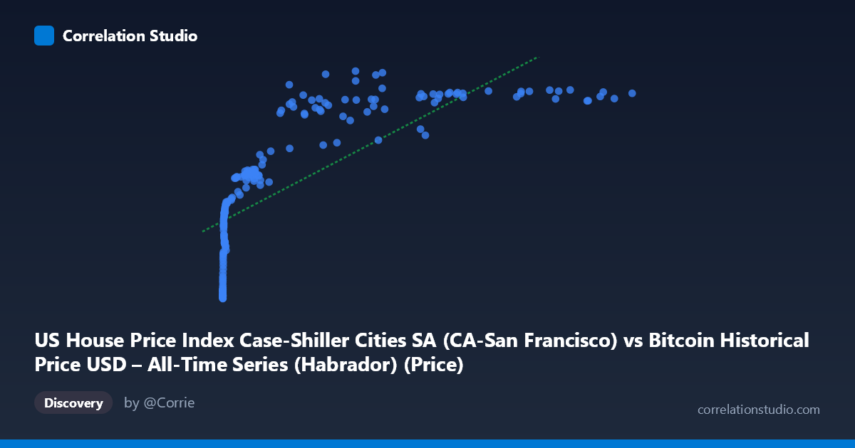
US House Price Index Case-Shiller Cities SA (CA-San Francisco) vs Bitcoin Historical Price USD – All-Time Series (Habrador) (Price)
- Pearson correlation (r)
- 0.7512
- Spearman correlation
- 0.9615
- p-value
- 0
- Sample size (n)
- 187
- 95% confidence interval
- 0.6812 to 0.8077
- Granger causality
- None
- Granger optimal lag
- 9
AI analysis
Analysis: Bitcoin Price vs. Case-Shiller SF Home Price Index
1. What the Visualization Reveals
The scatterplot shows a clear positive but strongly non-linear relationship between Bitcoin's USD price (X-axis) and the Case-Shiller San Francisco home price index (Y-axis). The data traces a logarithmic-like curve: Y rises steeply as X moves from near-zero to a few thousand dollars, then flattens into a much shallower slope as X extends into the tens of thousands and beyond. For example, moving from X≈3 to X≈1,000 corresponds to Y climbing from ~130 to ~235 (a huge jump), while moving from X≈20,000 to X≈118,000 only lifts Y from ~330 to ~360. This compression at high X values is the classic signature of a log-linear relationship rather than a straight-line one.
2. Strength, Direction, and Uncertainty
The Pearson correlation (r = 0.751, r² = 0.564) indicates a strong positive linear association, with the linear model explaining about 56% of the variance in Y. The 95% CI [0.681, 0.808] is reasonably tight and excludes zero, and the p-value of ~0 confirms this correlation is highly statistically significant — not a chance artifact of sampling. However, the note that Spearman's ρ exceeds Pearson's r is important: it tells us the rank-order relationship is even stronger than the linear fit suggests, reinforcing that a log or power-law transformation of X would likely produce a substantially better fit (probably r² well above 0.7–0.8). Critically, the Granger causality tests show no significant predictive direction in either direction (X→Y: p=0.72; Y→X: p=0.76) at the optimal lag of 9 periods. This means neither series helps forecast the other's future values — the correlation is contemporaneous/structural, not a lead-lag causal relationship in the time-series sense.
3. Notable Patterns and Outliers
Three broad regimes are visible: (a) a dense cluster of very early, very low Bitcoin prices (X < 20) paired with Y in the 128–155 range, representing 2010-era data; (b) a mid-range zone (X = 100–10,000) where Y climbs rapidly through the 170–270 range; and (c) a high-X plateau (X 20,000) where Y compresses into a narrow 300–380 band despite X varying by an order of magnitude. Some scatter/noise exists in the plateau — e.g., points like (45092, 306) and (29111, 300) sit noticeably below neighboring points at similar X values (e.g., 44354→379, 34855→332), suggesting Bitcoin price alone doesn't fully determine the housing index level at any given time, likely reflecting the independent timing of each series' own cycles.
4. Confounding Factors and Caveats
This is almost certainly a spurious-by-construction correlation driven by shared time trends rather than any economic mechanism linking Bitcoin price to SF home prices. Both series have risen dramatically over the 2010–2026 window due to entirely different drivers (crypto speculation/adoption vs. real estate/monetary policy, Fed rate cycles, SF tech-sector wealth). Any two monotonically-trending time series will show high correlation and r² simply from being aligned in time (a classic "trending time series" fallacy). The lack of Granger causality further supports this — there's no evidence of a genuine predictive/causal link, only co-movement over a shared temporal trend. Additionally, mismatched sampling frequency (n=187 paired vs. N=470 total) and the extreme right-skew of X (mean 20,037 vs. median far lower, stdev 29,663) mean a handful of high-X points exert outsized leverage on the linear fit.
5. Actionable Insights
- Refit non-linearly: Given the note on Spearman Pearson, fit log(X) vs. Y or a power/log-log model — this should substantially raise explained variance and better reflect the visible curve shape. - Detrend before concluding causality: Apply differencing or use growth rates (% change) rather than levels for both series to remove the shared upward trend, then re-test correlation and Granger causality — this is the standard fix for spurious time-series correlation. - Treat this as coincidental co-trending, not a tradable/causal signal: given no Granger causality, don't use Bitcoin price to forecast SF housing (or vice versa) in this raw form. - Add control variables: incorporate macro variables (interest rates, M2 money supply, tech-sector employment/stock indices) that plausibly drive both series, to test whether the correlation survives as a partial correlation.
X dataset: Bitcoin Historical Price USD – All-Time Series (Habrador)
Y dataset: US House Price Index Case-Shiller Cities SA
Part of experiment: Bitcoin - Bitcoin Historical Price USD – All-Time Series (Habrador) vs US House Price Index Case-Shiller Cities SA