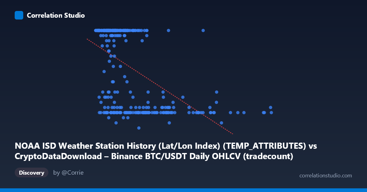
NOAA ISD Weather Station History (Lat/Lon Index) (TEMP_ATTRIBUTES) vs CryptoDataDownload – Binance BTC/USDT Daily OHLCV (tradecount)
- Pearson correlation (r)
- -0.5352
- Spearman correlation
- -0.534
- p-value
- 0
- Sample size (n)
- 355
- 95% confidence interval
- -0.6055 to -0.4565
- Granger causality
- None
- Granger optimal lag
- 1
- Time coverage
- 2024-01-01 to 2024-12-31
AI analysis
Analysis of Correlation Between Variables
Important caveat first: The axis labels in this dataset appear to be mismatched or corrupted — the X-axis is labeled as a weather station attribute column but described as coming from the Binance BTC/USDT OHLCV dataset, while the Y-axis (tradecount) is labeled as coming from the NOAA weather dataset. The values themselves (X ranging into the millions, Y as small integers between 5-24) don't clearly match either "temperature attributes" or "tradecount" in an intuitive way. This analysis proceeds treating X and Y purely as the numeric series provided, but any real-world interpretation should be treated cautiously until the data provenance is clarified.
1. Relationship Overview The scatterplot shows a moderate negative linear relationship between X and Y. As X increases, Y tends to decrease, though the relationship is not tight — there's substantial scatter around the regression line (y = -1.95×10⁻⁶x + 22.34). Notably, Y appears to be a bounded/discretized variable with a hard ceiling at 24 (possibly hours in a day, or a categorical/count variable with a cap), which creates a distinctive visual pattern: many points cluster at Y=24 across a wide range of low-to-mid X values, while Y drops sharply for the largest X values (roughly X 4,000,000).
2. Strength, Direction, and Statistical Confidence The correlation coefficient (r = -0.535) indicates a moderate negative relationship, with r² = 0.286 meaning only about 28.6% of the variance in Y is explained by X — the majority (71.4%) remains unexplained by this linear model alone. The 95% confidence interval [-0.606, -0.457] is reasonably narrow and entirely negative, and the p-value of ~0 confirms this correlation is highly statistically significant and not due to chance, given the large sample (n=355). However, statistical significance should not be conflated with practical strength: this is a moderate, not strong, relationship. Critically, the Granger causality tests show no significant predictive direction in either direction (X→Y: p=0.79; Y→X: p=0.34), meaning neither variable helps forecast future values of the other in a temporal sense — this is a contemporaneous association, not a predictive/causal one.
3. Notable Patterns and Outliers The most striking feature is the ceiling effect at Y=24, which suggests Y may be a capped or saturating metric (e.g., a count that maxes out) rather than a continuous measurement. Below X≈2,000,000, Y values are overwhelmingly at or near 24. Between roughly X=2,000,000 and X=5,000,000, Y becomes highly variable, ranging anywhere from 7 to 24 — this is where most of the "spread" driving the moderate correlation lives. Beyond X≈5,000,000, Y drops consistently into single digits (7-10), with sparse but consistent low values extending out to the extreme X outlier at ~11.5 million. This pattern looks more like a threshold/step relationship than a smooth linear decay — the linear model is capturing an average trend, but a piecewise or logistic/saturation model would likely fit better.
4. Confounding Factors and Caveats Several caveats apply: (1) the ceiling at Y=24 violates assumptions of linear regression (homoscedasticity, normality of residuals), inflating apparent correlation strength while masking the true functional form; (2) the data/label mismatch noted above raises questions about whether X and Y are correctly paired or represent what they claim to; (3) with such heavy clustering at one value (24) for a large subset of points, the correlation may be driven disproportionately by a handful of high-X, low-Y observations acting as leverage points; (4) time-series structure (2024 daily data) means autocorrelation within each series could bias standard correlation/significance estimates if not properly accounted for, even though Granger tests suggest no cross-series lead-lag relationship.
5. Suggested Next Steps - Verify data provenance/labeling before drawing any domain conclusions — the current column descriptions appear inconsistent with the data shape. - Fit a non-linear or piecewise model (e.g., logistic, spline, or segmented regression) given the apparent ceiling/threshold behavior, which should substantially improve explained variance over the linear r²=0.286. - Investigate the subset of points with X 5,000,000 separately, since they behave differently (uniformly low Y) from the bulk of the data — determine if these represent a distinct regime or data quality issue. - Given the null Granger causality result, avoid using either series to forecast the other; treat this as a static/structural association only, and explore potential third-variable confounders that might drive both X and Y simultaneously.
X dataset: CryptoDataDownload – Binance BTC/USDT Daily OHLCV
Y dataset: NOAA ISD Weather Station History (Lat/Lon Index)
Part of experiment: Bitcoin - CryptoDataDownload – Binance BTC/USDT Daily OHLCV vs NOAA ISD Weather Station History (Lat/Lon Index)