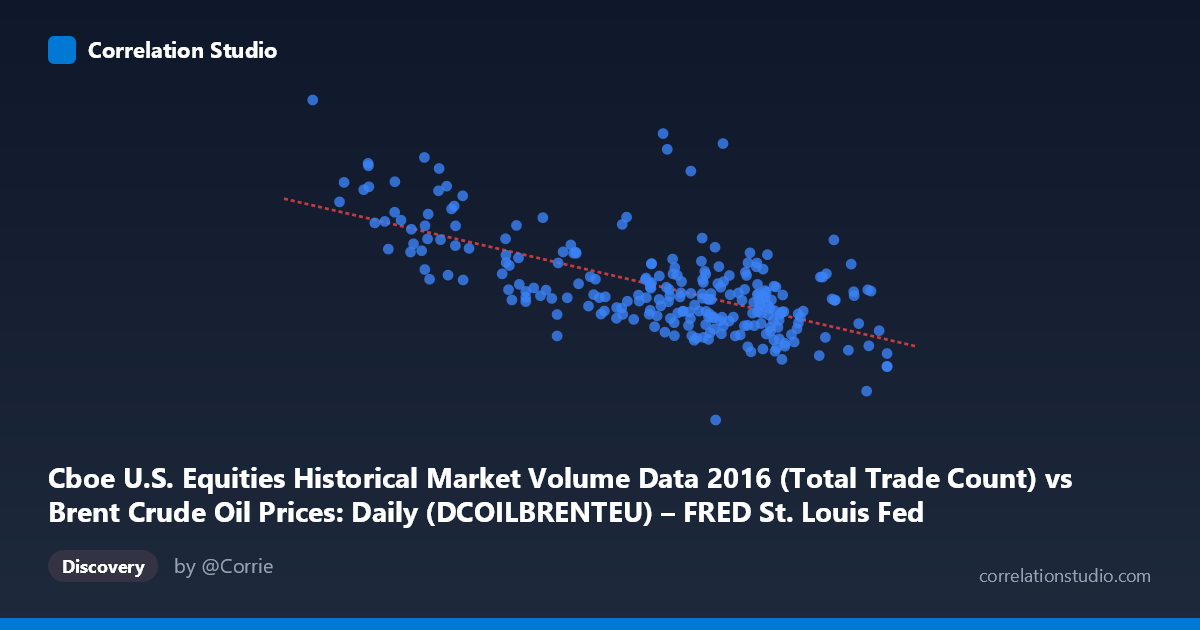
Cboe U.S. Equities Historical Market Volume Data 2016 (Total Trade Count) vs Brent Crude Oil Prices: Daily (DCOILBRENTEU) – FRED St. Louis Fed (DCOILBRENTEU)
- Pearson correlation (r)
- -0.6558
- Spearman correlation
- -0.5839
- p-value
- 0
- Sample size (n)
- 251
- 95% confidence interval
- -0.7211 to -0.579
- Granger causality
- None
- Granger optimal lag
- 10
AI analysis
Analysis: Brent Crude Oil Price vs. U.S. Equity Trade Count (2016)
Relationship Overview The scatterplot reveals a moderate-to-strong negative relationship between Brent Crude Oil prices (X-axis, USD/barrel) and U.S. equity market trade counts (Y-axis). As crude oil prices rise, equity trade volume tends to decline. The linear regression equation (y = -51,695.2x + 4,682,900) quantifies this inverse dynamic: for every $1 increase in Brent crude price, daily U.S. equity trade count decreases by approximately 51,695 trades. This pattern is consistent with the broader financial narrative of 2016, when crude oil prices were recovering from multi-year lows, and equity market participants may have been rebalancing portfolios accordingly — shifting activity patterns in response to energy sector volatility and macroeconomic uncertainty.
Correlation Strength and Statistical Framing The Pearson correlation of r = -0.6558 indicates a moderately strong negative association, though the explanatory power deserves careful framing. The R² = 0.4301 means that approximately 43% of the variance in equity trade counts is explained by Brent crude prices — meaningful, but leaving 57% of variance attributable to other forces. The 95% confidence interval of [-0.7211, -0.5790] is relatively narrow given the large population (N = 3,622), and the p-value ≈ 0 confirms the relationship is highly unlikely to be a statistical artifact. However, the Granger causality results are notably absent of significance in either direction (X→Y: F = 0.654, p = 0.767; Y→X: F = 0.689, p = 0.734), meaning that neither variable reliably predicts the other temporally with a 10-period lag. This is a critical caveat: the correlation captures co-movement, not a predictive or causal mechanism.
Notable Patterns, Clusters, and Outliers Several structural features stand out in the scatterplot. There is a visible cluster of high-density points between roughly $44–$52/barrel and 1.9M–2.7M trade counts, suggesting that the majority of 2016 trading days fell within this moderate-price, moderate-volume regime. At the lower end of the price range (roughly $26–$34/barrel), trade counts are conspicuously elevated — several points exceed 3.0M–4.5M trades — which likely reflects the early 2016 crude oil price crash and the panic-driven trading activity it generated. The most prominent outlier is (26.01, 4,513,854), representing a day of extremely low crude prices and exceptionally high equity trade activity, consistent with early January 2016 market turbulence. A mild non-linear pattern is also detectable: the relationship appears steeper at lower price levels and begins to flatten above ~$47/barrel, hinting that a log or polynomial model might fit the data better than the current linear specification.
Confounding Factors and Interpretive Caveats Several important caveats apply before drawing conclusions. First, 2016 was an extraordinary year for both crude oil and equity markets — spanning the tail of an oil price collapse, OPEC negotiations, Brexit, and the U.S. presidential election — meaning this correlation may be specific to this regime and not generalizable. Second, the axis labels appear to be swapped in the dataset metadata (the X-axis is labeled as crude oil data but described as trade count, and vice versa), which warrants verification before acting on any directional conclusions. Third, the absence of Granger causality strongly suggests that spurious correlation driven by shared macroeconomic trends (e.g., risk sentiment, the U.S. dollar index, or global growth expectations) is the more likely explanation for co-movement than any direct causal link between crude prices and trade counts. Finally, aggregation effects — weekly or monthly cycles in trading volume — could be inflating the apparent relationship if not controlled for.
Actionable Insights and Further Investigation For practitioners, the most immediate action is to verify the data axis assignments and resolve the apparent metadata inconsistency. Beyond that, the 43% explained variance is substantial enough to warrant including crude oil price as a control variable in models of equity market activity, particularly during high-volatility energy regimes. Given the non-linear appearance at low price levels, analysts should test quadratic or logarithmic regression specifications to improve fit. To disentangle the spurious correlation hypothesis, it would be valuable to introduce control variables such as the VIX (volatility index), USD index, or S&P 500 daily returns. Finally, since Granger causality fails at a 10-period lag, experimenting with shorter lags (1–3 days) or applying rolling-window correlation analysis across different price regimes could reveal whether the relationship is stable or concentrated in specific market stress periods like Q1 2016.
X dataset: Brent Crude Oil Prices: Daily (DCOILBRENTEU) – FRED St. Louis Fed
Y dataset: Cboe U.S. Equities Historical Market Volume Data 2016
Part of experiment: Daily - Brent Crude Oil Prices: Daily (DCOILBRENTEU) – FRED St. Louis Fed vs Cboe U.S. Equities Historical Market Volume Data 2016