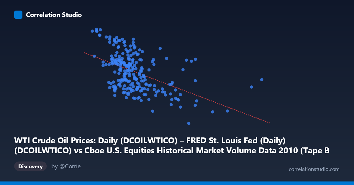
WTI Crude Oil Prices: Daily (DCOILWTICO) – FRED St. Louis Fed (Daily) (DCOILWTICO) vs Cboe U.S. Equities Historical Market Volume Data 2010 (Tape B Notional)
- Pearson correlation (r)
- -0.4909
- Spearman correlation
- -0.475
- p-value
- 0
- Sample size (n)
- 252
- 95% confidence interval
- -0.5793 to -0.391
- Granger causality
- None
- Granger optimal lag
- 1
AI analysis
Scatterplot Analysis: WTI Crude Oil Prices vs. Cboe Tape B Notional Volume (2010)
Relationship Overview
The scatterplot reveals a moderate negative relationship between WTI crude oil prices (X-axis) and Cboe Tape B notional trading volume (Y-axis) across 252 trading days in 2010. As oil prices increase, equity notional volume on Tape B tends to decline. The linear regression equation (y = −1.27×10⁻⁹x + 86.04) confirms this inverse slope, though the scatter around the regression line is substantial, suggesting oil price alone is far from a complete explanation of volume dynamics. The relationship is visible but noisy — many data points deviate considerably from the trend line, particularly in the mid-range of oil prices.
Correlation Strength, Direction, and Statistical Significance
The Pearson correlation of r = −0.4909 indicates a moderate negative association. More importantly, the coefficient of determination r² = 0.2410 means only ~24% of the variance in Tape B notional volume is explained by WTI crude oil prices — leaving roughly 76% attributable to other factors entirely. The 95% confidence interval [−0.5793, −0.3910] is meaningfully away from zero and relatively tight given the sample size (n = 252), and the p-value of effectively 0 confirms this correlation is highly statistically significant and unlikely to be a sampling artifact, particularly with a population of N = 3,302. However, statistical significance does not imply practical magnitude, and the r² cautions against over-interpreting the relationship as strongly predictive.
Patterns, Clusters, and Outliers
Several notable structural features emerge from the data. A dense cluster of observations sits between roughly $3–6 billion in oil price units and 74–87 in Tape B notional, forming the core of the negative trend. However, there are visible high-leverage outliers at extreme X values — for instance, points near X ≈ 15.1B (75.10) and X ≈ 15.96B exhibit elevated oil prices with relatively average or low volumes, pulling the regression line. On the low-oil-price end, several points (e.g., X ≈ 2.0B, Y = 90.84; X ≈ 2.26B, Y = 89.83) show notably high Tape B volume, consistent with the negative trend but also suggesting possible elevated volatility periods. There is also a suggestion of heteroscedasticity — variance in Y appears wider at lower X values and compresses somewhat at higher X values — which could affect the reliability of standard linear regression assumptions.
Confounding Factors and Interpretive Caveats
Several important caveats apply. First, the axis labels appear to be swapped relative to their dataset descriptions — WTI crude oil prices in USD per barrel should realistically range from ~$70–$95 in 2010, yet the X-axis shows values in the billions, which aligns more with notional trading volume; this warrants careful verification of the data mapping before drawing firm conclusions. Second, no significant Granger causality was detected in either direction (X→Y: F=1.23, p=0.27; Y→X: F=3.29, p=0.07), meaning neither variable reliably predicts the future values of the other at a 1-period lag — the observed correlation may reflect concurrent macroeconomic drivers (e.g., risk-off sentiment, economic uncertainty, Federal Reserve policy in 2010) rather than any direct causal mechanism. Third, 2010 was a specific macro environment featuring post-financial-crisis recovery and the Deepwater Horizon oil spill, which could create period-specific spurious correlations not generalizable to other years.
Actionable Insights and Further Investigation
Given the 76% unexplained variance, further investigation should focus on additional covariates: VIX (volatility index), S&P 500 returns, macroeconomic announcements, and sector-specific flows would likely account for much of the residual variance. The near-significant Y→X Granger result (p=0.071) is worth revisiting with longer lag structures or a VAR model — it hints that equity volume may have weak leading predictive content for oil prices that a single lag fails to capture fully. Analysts should also segment the data by market regime (e.g., high-volatility vs. low-volatility periods) to determine whether the negative correlation is consistent throughout 2010 or driven by specific episodes. Finally, resolving the suspected axis-labeling discrepancy is a prerequisite for any actionable use of this analysis in trading or risk management contexts.
X dataset: Cboe U.S. Equities Historical Market Volume Data 2010
Y dataset: WTI Crude Oil Prices: Daily (DCOILWTICO) – FRED St. Louis Fed (Daily)
Part of experiment: Daily - Cboe U.S. Equities Historical Market Volume Data 2010 vs WTI Crude Oil Prices: Daily (DCOILWTICO) – FRED St. Louis Fed (Daily)