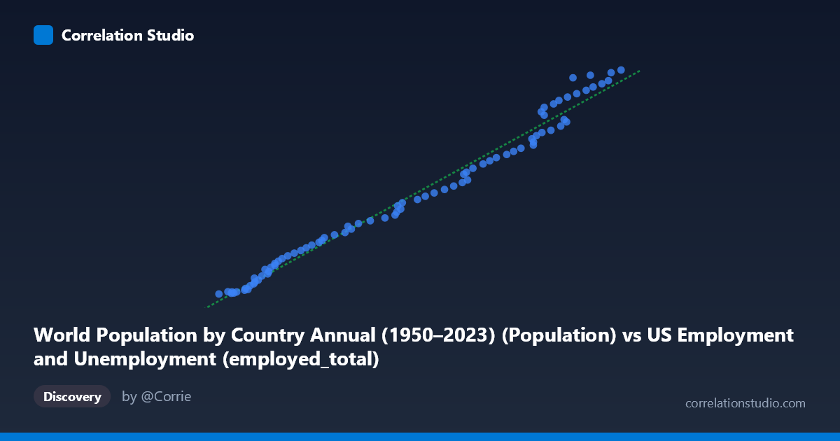
World Population by Country Annual (1950–2023) (Population) vs US Employment and Unemployment (employed_total)
- Pearson correlation (r)
- 0.9915
- Spearman correlation
- 0.9971
- p-value
- 0
- Sample size (n)
- 83
- 95% confidence interval
- 0.9868 to 0.9945
- Granger causality
- None
- Granger optimal lag
- 10
- Time coverage
- 1941-01-01 to 2023-01-01
AI analysis
Scatterplot Analysis: World Population vs. US Total Employment (1941–2023)
1. Nature of the Relationship
The scatterplot reveals a strikingly tight, positive, and nearly linear relationship between world population and total US employment over the period 1941–2023. As world population grows across the observed range (~50 million to ~161 million on the X-axis, likely representing a specific population segment or scaled metric), US total employed persons rise correspondingly from roughly 46 million to 163 million. The data points cluster closely around the regression line (y = 1,035.99x − 9,379,530), with very little visible scatter, suggesting an extraordinarily consistent co-movement across eight decades of data. This visual pattern immediately signals a near-perfect monotonic trend.
2. Correlation Strength, Direction, and Causality
The correlation is exceptionally strong and positive (r = 0.9915), with R² = 0.9830 indicating that 98.3% of the variance in US total employment is statistically explained by world population. The 95% confidence interval [0.9868, 0.9945] is extremely narrow, confirming this is a highly stable and precisely estimated relationship, not an artifact of small-sample noise (n = 83). The p-value of effectively zero reinforces that this association is statistically indistinguishable from certainty under conventional thresholds. However — and critically — Granger causality tests find no significant predictive directionality in either direction (X→Y: F = 1.20, p = 0.31; Y→X: F = 1.15, p = 0.34), even at an optimal lag of 10 periods. This means that past values of world population do not reliably predict future US employment beyond what is already known, and vice versa. The correlation is real but temporally non-causal in the Granger sense.
3. Patterns, Clusters, and Outliers
The data points distribute fairly evenly along the regression line without obvious clustering into discrete groups, which is consistent with two variables that both increase smoothly over time. A few points at the upper end of the range (X 145,000; Y 145 million) show slightly more scatter around the fitted line, with some observations appearing marginally above and below the trend — suggesting that in recent decades the relationship may be very mildly heteroscedastic or that episodic disruptions (e.g., the COVID-19 labor market shock around 2020) introduced brief deviations. There are no dramatic outliers that visually break from the linear trend, though the uppermost cluster warrants closer inspection given that the 2020–2022 period was highly anomalous for employment.
4. Confounding Factors and Critical Caveats
This correlation almost certainly reflects shared time-trend confounding rather than any meaningful structural link between world population and US employment. Both variables are non-stationary time series that trend upward across the 20th and early 21st centuries; nearly any two monotonically increasing global indicators measured over this period would correlate at similarly extreme levels (a classic spurious regression problem). The dataset labeling itself raises red flags — "World Population" appears in the US Employment dataset and vice versa, suggesting possible metadata misattribution. Furthermore, US employment is driven by domestic demographic factors (working-age population, labor force participation), business cycles, policy, and technology — none of which are directly governed by global headcount. The Granger non-causality result is consistent with this interpretation: the co-movement is a temporal coincidence, not a dynamic feedback system.
5. Actionable Insights and Further Investigation
Given the near-certain spuriousness of this correlation, the most important next step is detrending both series (e.g., first-differencing or applying Hodrick-Prescott filtering) before drawing any analytical conclusions — the residual correlation after removing shared time trends would be far more informative. Researchers should also verify the dataset column assignments, as the variable labeling appears inverted between datasets. If a genuine structural relationship is hypothesized (e.g., global labor supply affecting US employment through trade or migration channels), more appropriate analyses would include cointegration testing (Engle-Granger or Johansen), vector error correction models, or cross-correlation of stationary residuals. Finally, segmenting the analysis by decade or economic regime (pre/post-globalization, pre/post-automation) could reveal whether the relationship strengthens or weakens in meaningful ways that the aggregate 83-year trend obscures.
X dataset: US Employment and Unemployment
Y dataset: World Population by Country Annual (1950–2023)
Part of experiment: Yearly - US Employment and Unemployment vs World Population by Country Annual (1950–2023)