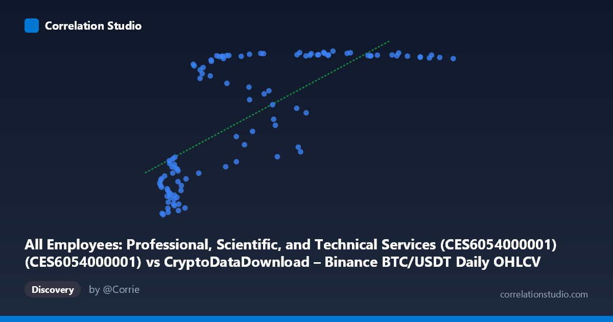
All Employees: Professional, Scientific, and Technical Services (CES6054000001) (CES6054000001) vs CryptoDataDownload – Binance BTC/USDT Daily OHLCV (Close)

Pearson correlation (r): 0.7248
Spearman correlation: 0.8073
p-value: 0
Sample size (n): 106
95% confidence interval: 0.6198 to 0.8044
Granger causality: None
Granger optimal lag: 10
Time coverage: 2017-09-01 to 2026-06-01
Recomputed on refreshed data: 2026-10-10 (r was 0.7218)

AI analysis

Analysis: Employment Levels vs. BTC/USDT Price

1. What the Visualization Reveals

The scatterplot shows a strongly non-linear, saturating relationship rather than a clean linear trend. At low X-values (roughly 3,000–20,000, corresponding to employment counts), Y (BTC price) is compressed in a narrow band around 9,100–9,700. As X increases past ~20,000, Y jumps sharply and then plateaus at a high level (~10,750–10,820) for the remainder of the range, with only minor fluctuations. This produces a curve shape more like a step-function or logarithmic/logistic rise than a straight line — most of the "action" happens in a relatively narrow X-band before Y flattens out.

2. Strength, Direction, and Statistical Meaning

The Pearson correlation (r = 0.72, r² = 0.52) indicates a strong positive linear association, with the linear model explaining about 52% of Y's variance. The 95% CI [0.615, 0.802] is reasonably tight and excludes zero, and the p-value ≈ 0 confirms this correlation is highly unlikely to be due to chance. However, r² of 0.52 also means nearly half the variance in Y is unexplained by a linear fit — consistent with the visibly non-linear, plateauing pattern described above, which a straight-line model captures only partially. Critically, the Granger causality tests show no significant predictive direction either way (X→Y: p=0.60; Y→X: p=0.55) at the optimal lag of 10 periods. This means despite the strong contemporaneous correlation, neither series reliably helps forecast the other's future values — the relationship is associative, not (Granger-)causal or lead-lag in nature.

3. Notable Patterns and Features

- Two-regime structure: a "low-X/low-Y" cluster (X < 20,000, Y ~9,100–9,700) and a "high-X/high-Y" plateau (X 40,000, Y ~10,700–10,820), with a transition zone between ~20,000–50,000 where Y rises steeply and shows the most scatter (e.g., points like (48810, 10044.8), (49587, 9710.4), (29331, 9603.8) deviate from the otherwise tight plateau). - Saturation/ceiling effect: Y appears bounded near 10,820 regardless of how large X gets (X ranges up to 118,595), suggesting Y (employment) has structurally limited upside — plausible for a labor-market series with slow, bounded growth compared to BTC price's multiplicative swings. - Outliers in the transition zone: several mid-X points fall well below the plateau trend, indicating instability or regime-dependent behavior during the transition period rather than smooth monotonic increase.

4. Confounding Factors and Caveats

The most important caveat: this pairing conflates a daily financial time series (BTC/USDT price) with a monthly macroeconomic series (professional services employment), aligned only via resampling/interpolation. Both series likely share a common confound — time itself (secular trend/growth over 2017–2026) — rather than any direct economic mechanism linking crypto prices to professional-services hiring. This is a classic spurious-correlation risk: two upward-trending series over the same multi-year window will correlate strongly even absent any causal link. The lack of Granger causality reinforces that this is likely a shared-trend artifact rather than a genuine predictive relationship. Additionally, employment data are seasonally adjusted and monthly (low frequency, ~105 effective points) while BTC data are daily — the frequency mismatch and interpolation could artificially smooth or inflate the apparent correlation.

5. Suggestions for Further Investigation

- Detrend both series (e.g., first-differencing, or regressing out a time trend) and recheck correlation — if r drops substantially, this confirms the relationship is trend-driven rather than substantive. - Fit a non-linear model (logistic, log, or piecewise) given the visible saturation pattern; this should outperform the linear r²=0.52 and better represent the true functional form. - Explore whether a third variable (e.g., overall GDP growth, stock market indices, or general risk-asset sentiment) drives both series independently. - Given no Granger causality, avoid using either series to forecast the other; instead treat the correlation as descriptive/contextual only, not predictive. - Consider narrowing the analysis window or matching frequency (e.g., using BTC monthly averages) to reduce noise and test robustness of the relationship.

X dataset: CryptoDataDownload – Binance BTC/USDT Daily OHLCV

Y dataset: All Employees: Professional, Scientific, and Technical Services (CES6054000001)

Part of experiment: Bitcoin - CryptoDataDownload – Binance BTC/USDT Daily OHLCV vs All Employees: Professional, Scientific, and Technical Services (CES6054000001)