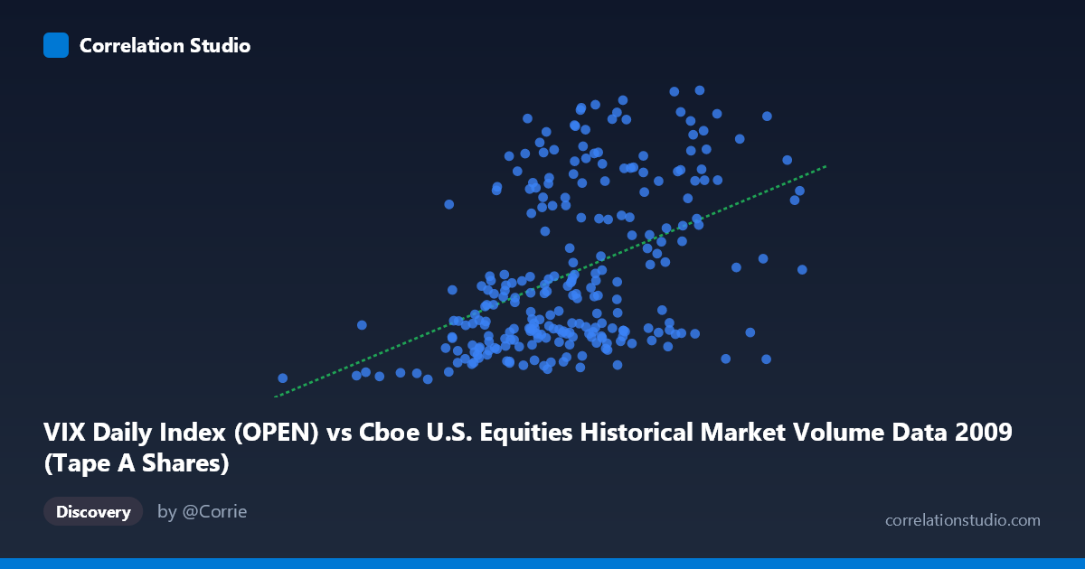
VIX Daily Index (OPEN) vs Cboe U.S. Equities Historical Market Volume Data 2009 (Tape A Shares)
- Pearson correlation (r)
- 0.444
- Spearman correlation
- 0.4474
- p-value
- 0
- Sample size (n)
- 252
- 95% confidence interval
- 0.339 to 0.538
- Granger causality
- None
- Granger optimal lag
- 1
AI analysis
Scatterplot Analysis: VIX Open vs. Tape A Shares (2009)
Relationship Overview
The scatterplot reveals a moderate positive relationship between the Cboe VIX Daily Index (Open) on the X-axis and Tape A Share volume on the Y-axis across the 2009 trading year. As VIX open values increase — reflecting higher anticipated market volatility — Tape A share volumes tend to rise as well. This is economically intuitive: elevated fear or uncertainty (as measured by VIX) typically drives heightened trading activity, as market participants reposition portfolios, hedge exposures, or react to news events. The linear regression equation (y = 4.17×10⁻⁸x + 13.43) confirms this positive slope, though the relatively small coefficient on X signals that volume gains per unit of VIX increase are modest.
Correlation Strength and Statistical Significance
The Pearson correlation of r = 0.444 indicates a moderate positive association, but the more telling metric is r² = 0.197: only about 19.7% of the variance in Tape A Share volume is explained by VIX open levels. The remaining ~80% is driven by other factors entirely. The 95% confidence interval of [0.339, 0.538] is reasonably tight and does not cross zero, lending confidence to the direction of the effect, and the p-value of 1.35×10⁻¹³ confirms this relationship is highly unlikely to be a statistical artifact given the sample of 252 paired observations drawn from a population of 3,232. That said, statistical significance here is partly a function of sample size — significance does not imply practical magnitude, and the modest r² underscores real limits in predictive power.
Granger Causality and Temporal Direction
Despite the statistically significant contemporaneous correlation, the Granger causality tests find no significant predictive directionality in either direction at a 1-period lag (X→Y: F = 0.519, p = 0.472; Y→X: F = 1.123, p = 0.290). This is a critical nuance: knowing yesterday's VIX open does not meaningfully help predict today's Tape A volume beyond baseline, and vice versa. The relationship appears to be contemporaneous rather than predictive — both variables likely respond simultaneously to the same underlying market conditions rather than one leading the other. This effectively rules out using either series as a reliable leading indicator of the other.
Notable Patterns, Clusters, and Outliers
The sample points reveal considerable dispersion rather than a tight linear band, consistent with the modest r². Several clusters are visible: a dense grouping of lower-VIX, lower-volume observations (roughly X: 300M–500M, Y: 20–30) likely corresponding to calmer mid-year 2009 market conditions, and a more scattered upper cluster of higher VIX/higher volume points (Y: 40–52) that may correspond to residual volatility from the post-financial-crisis environment early in 2009. Notable outliers include points such as (663M, 49.68) and (606M, 49.96), which show very high volume and high VIX simultaneously, and conversely (644M, 24.91) and (662M, 21.84), which show high X values with surprisingly low Y — suggesting the relationship breaks down at extreme X values. This heteroscedasticity (wider Y spread at higher X) hints at non-linear dynamics.
Caveats, Confounders, and Further Investigation
Several confounding factors deserve attention. 2009 is a structurally unusual year: markets were recovering from the 2008 financial crisis, meaning VIX levels and volumes were both elevated by macro regime effects that co-determined both variables simultaneously. Seasonal trading patterns, index rebalancing events, and earnings seasons could independently drive volume spikes uncorrelated with VIX. The axis labeling also warrants scrutiny — the dataset notes suggest a possible column assignment inversion (VIX data appears in a market volume dataset field and vice versa), which should be verified before drawing firm conclusions. For further investigation, analysts should: (1) test non-linear models (log or polynomial) given visible heteroscedasticity; (2) segment by market regime (e.g., pre/post March 2009 market bottom); (3) incorporate additional predictors such as S&P 500 returns, bid-ask spreads, or macro announcements to explain the remaining 80% of variance; and (4) validate column sourcing to ensure the variable assignments are correctly matched across datasets.
X dataset: Cboe U.S. Equities Historical Market Volume Data 2009
Y dataset: VIX Daily Index
Part of experiment: Daily - Cboe U.S. Equities Historical Market Volume Data 2009 vs VIX Daily Index