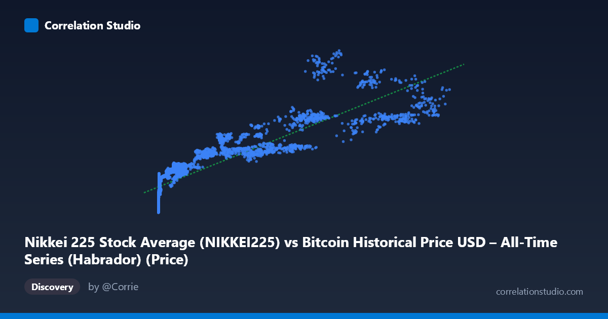
Nikkei 225 Stock Average (NIKKEI225) vs Bitcoin Historical Price USD – All-Time Series (Habrador) (Price)
- Pearson correlation (r)
- 0.8723
- Spearman correlation
- 0.9639
- p-value
- 0
- Sample size (n)
- 3860
- 95% confidence interval
- 0.8646 to 0.8797
- Granger causality
- None
- Granger optimal lag
- 10
AI analysis
Analysis: Nikkei 225 vs. Bitcoin Price Relationship
1. What the Visualization Reveals
The scatterplot shows a strong positive, but distinctly non-linear relationship between the Nikkei 225 index (X) and Bitcoin price (Y). At low X-values (near zero, representing early Nikkei/Bitcoin history), Y clusters tightly between ~8,000–15,000. As X increases, Y rises steadily but with increasing dispersion, and the relationship appears to curve — consistent with a logarithmic or power-law shape rather than a strictly linear one. The linear fit (y = 0.303x + 16,483) captures the broad upward trend but likely underfits the compressed low-X cluster and overfits variance at high X, where scatter widens substantially (e.g., Bitcoin values ranging from ~25,000 to ~55,000 at similar Nikkei levels around 39,000–68,000).
2. Strength, Direction, and Statistical Confidence
The correlation coefficient (r = 0.872) indicates a strong positive linear association, with r² = 0.761 meaning roughly 76% of the variance in Bitcoin price is statistically explained by Nikkei 225 levels — a substantial share, though nearly a quarter of variance remains unexplained by this single variable. The 95% CI [0.865, 0.880] is tight, and p ≈ 0 confirms this correlation is highly unlikely to be due to chance given the large sample (n=3,860). However, the Granger causality tests reveal a critical caveat: neither direction (Nikkei→Bitcoin: F=1.30, p=0.227; Bitcoin→Nikkei: F=0.63, p=0.792) shows significant predictive causality at 10 lags. This strongly suggests the correlation is not causal in a temporal/predictive sense — both series likely trend together due to shared macro drivers (e.g., global liquidity, risk sentiment, time itself) rather than one leading the other.
3. Notable Patterns and Outliers
A dense cluster near X≈0–1,000 with Y≈8,000–20,000 represents early-era data where Bitcoin was in its infancy and Nikkei data may have limited variation or represents a rebased/early index period — this cluster disproportionately influences the correlation given its density. Above X≈40,000, dispersion increases sharply: points like (68,111, 55,621) and (66,011, 38,815) sit far above the regression line, while (58,102, 29,518) sits below, suggesting Bitcoin's explosive rallies (2020-21, 2024-25) create outliers not well captured by Nikkei movements. This heteroscedasticity (fanning pattern) is a classic sign that a simple linear model is inadequate for the full range.
4. Confounding Factors and Caveats
The most significant concern is that both series may simply share a common time trend rather than any genuine economic relationship — both Bitcoin and global equity indices have broadly risen over the 2010–2026 window due to unrelated secular forces (monetary expansion, adoption growth, inflation). This is a classic spurious correlation risk with non-stationary time series. The absence of Granger causality reinforces this: if Nikkei truly drove Bitcoin (or vice versa), we'd expect predictive power in at least one direction. Additionally, comparing an equity index (bounded, mean-reverting-ish) to Bitcoin (unbounded, multiplicative growth) mismatches the data-generating processes, inflating apparent correlation through shared upward drift alone.
5. Actionable Insights and Next Steps
Given the lack of Granger causality, this correlation should not be used for predictive trading signals in either direction. Instead: (a) test correlation on differenced/returns data (% change) rather than levels, which removes trend-driven spurious correlation and reveals true co-movement; (b) apply cointegration tests (e.g., Engle-Granger) to check for a genuine long-run equilibrium relationship despite non-causality; (c) introduce a common macro variable (e.g., USD index, real rates, global M2) as a control to test whether Nikkei and Bitcoin are both proxies for a third factor; and (d) consider log-transforming both axes, given Bitcoin's exponential growth pattern, to assess whether a log-log model fits substantially better than the current linear specification.
X dataset: Bitcoin Historical Price USD – All-Time Series (Habrador)
Y dataset: Nikkei 225 Stock Average
Part of experiment: Bitcoin - Bitcoin Historical Price USD – All-Time Series (Habrador) vs Nikkei 225 Stock Average