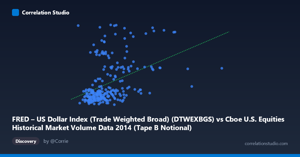
FRED – US Dollar Index (Trade Weighted Broad) (DTWEXBGS) vs Cboe U.S. Equities Historical Market Volume Data 2014 (Tape B Notional)
- Pearson correlation (r)
- 0.418
- Spearman correlation
- 0.464
- p-value
- 0
- Sample size (n)
- 245
- 95% confidence interval
- 0.3088 to 0.5163
- Granger causality
- None
- Granger optimal lag
- 1
AI analysis
Scatterplot Analysis: US Dollar Index vs. Cboe Tape B Notional Volume (2014)
Relationship Overview
The scatterplot reveals a modest positive relationship between the Trade Weighted Broad US Dollar Index (x-axis) and Cboe Tape B Notional trading volume (y-axis) across 245 trading days in 2014. The linear regression equation (y = 6.54×10⁻¹⁰x + 92.72) confirms a positive slope, suggesting that as dollar index values increase, Tape B notional volume tends to rise slightly. However, the relationship is far from clean — the scatter is substantial, with a notable concentration of points clustered in a relatively narrow x-range (~2.5B–6B) and y-range (~93–96), punctuated by a series of vertically dispersed high-y outliers that pull the regression line upward and are critical to understanding this correlation.
Correlation Strength and Statistical Significance
With r = 0.418 and r² = 0.175, the linear relationship explains only 17.5% of the variance in Tape B notional volume — meaning roughly 82.5% of variation is driven by other factors entirely. The 95% confidence interval for r of [0.309, 0.516] is meaningfully above zero and does not include zero, and the p-value of 8.88×10⁻¹² confirms this correlation is highly statistically significant given n = 245 and N = 3,686. However, statistical significance here should not be conflated with practical importance: the effect size is moderate at best. Critically, the Granger causality tests return no significant result in either direction (X→Y: F=0.12, p=0.73; Y→X: F=0.10, p=0.76), meaning neither variable temporally predicts the other at a one-period lag. This strongly undermines any causal narrative — the correlation likely reflects shared exposure to common macro drivers rather than a direct predictive relationship.
Notable Patterns, Clusters, and Outliers
The most striking visual feature is a dense horizontal cluster of points between approximately x = 2.5B–6B and y = 93–96, representing the bulk of "normal" trading days where both the dollar index and notional volume are relatively stable. Above this cluster, a scattered band of high-volume outliers (y ≈ 97–102+) appears across a wide x-range, suggesting episodic spikes in Tape B notional activity that do not correspond consistently to any particular dollar index level. Several extreme points — notably near x = 13B (far right) and x = 2.1B (far left), both with elevated y-values around 97–102 — appear to be highly influential leverage points that disproportionately shape the regression slope. The rightmost point (13B, ~97.35) is especially isolated and warrants scrutiny as a potential data anomaly or structural break.
Confounding Factors and Caveats
Several confounds complicate interpretation. First, both series are time-indexed to 2014, meaning any shared macro event — Federal Reserve communications, geopolitical shocks, or end-of-quarter rebalancing — could simultaneously move the dollar and equity trading volumes, producing spurious correlation. Second, Tape B notional volume is a narrow slice of total equity market activity (regional exchanges), making it sensitive to idiosyncratic microstructure events rather than broad macro forces. Third, the x-axis range is enormous (2.1B to 13B), with the distribution heavily right-skewed (mean ~4.4B, max ~13B), suggesting the data may not be well-described by a linear model. Finally, the axes appear to be swapped in labeling relative to the dataset descriptions (X contains the dollar index values, Y contains notional volume), which, while not analytically fatal, deserves verification before drawing conclusions.
Actionable Insights and Further Investigation
Given the weak explanatory power and absence of Granger causality, practitioners should not use the dollar index as a direct forecasting input for Tape B notional volume in a simple linear framework. Instead, the following steps are recommended: (1) Investigate the high-volume outlier days individually — identifying the specific dates and associated market events (e.g., FOMC meetings, macro data releases) could reveal whether these spikes are systematically event-driven; (2) Apply a log transformation to the x-variable given the extreme right skew and large dynamic range, which may improve linearity; (3) Test multi-factor models incorporating VIX (volatility), total market volume, and Fed policy event indicators as covariates to better isolate the dollar's marginal effect; and (4) Extend the time horizon beyond 2014 to test whether this correlation is regime-specific or structural, particularly given the dollar's significant trend moves in late 2014.
X dataset: Cboe U.S. Equities Historical Market Volume Data 2014
Y dataset: FRED – US Dollar Index (Trade Weighted Broad)
Part of experiment: Daily - Cboe U.S. Equities Historical Market Volume Data 2014 vs FRED – US Dollar Index (Trade Weighted Broad)