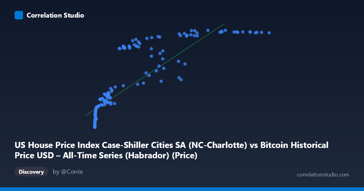
US House Price Index Case-Shiller Cities SA (NC-Charlotte) vs Bitcoin Historical Price USD – All-Time Series (Habrador) (Price)
- Pearson correlation (r)
- 0.8561
- Spearman correlation
- 0.9694
- p-value
- 0
- Sample size (n)
- 187
- 95% confidence interval
- 0.8124 to 0.8902
- Granger causality
- None
- Granger optimal lag
- 1
AI analysis
Analysis: Bitcoin Price vs. Charlotte Case-Shiller Home Price Index
1. What the Visualization Reveals
The scatterplot shows a clear positive but distinctly non-linear relationship between Bitcoin's historical price (X) and the Charlotte, NC Case-Shiller Home Price Index (Y). At low Bitcoin values (under $1,000), Y clusters tightly in the 110–150 range with little variation. As Bitcoin price climbs into the tens of thousands, Y rises more steeply but with increasing scatter, and the growth pattern resembles a logarithmic or saturating curve rather than a straight line — Y appears to compress toward an upper range (roughly 270–287) even as X spans a huge additional range (60,000 to 118,670).
2. Strength, Direction, and Uncertainty
The Pearson correlation (r = 0.856, r² = 0.733) indicates a strong positive linear association, with X statistically "explaining" about 73% of the variance in Y under a linear model. The 95% CI [0.812, 0.890] is tight and the p-value is effectively zero, so this correlation is highly unlikely to be due to sampling noise. However, strength of correlation should not be conflated with causation or mechanism — the Granger causality tests show no significant predictive direction in either direction (X→Y: p=0.29; Y→X: p=0.12) at a 1-period lag. This means neither series reliably "leads" the other in time — the relationship is more likely driven by a shared underlying trend (e.g., both series trending upward over the 2010–2026 window) rather than one variable causally forecasting the other.
3. Notable Patterns and Outliers
- Compression at both ends: Low-X points (Bitcoin under $100) show Y tightly bounded near 110–125, while high-X points (Bitcoin above $60,000) show Y compressed near 270–287 — suggesting a ceiling effect in the home price index or an early-adoption floor effect in Bitcoin. - Mid-range scatter: Between X ≈ 20,000–60,000, Y values are noticeably more dispersed (e.g., X=41,869→Y=213 vs. X=44,354→Y=245 vs. X=58,724→Y=197), indicating other factors modulate Y independent of Bitcoin price in this zone. - Non-monotonic patches: Some higher-X points yield lower Y than lower-X points (e.g., X=45,092→Y=194 vs. X=34,855→Y=209), hinting that time (not just Bitcoin price level) matters — likely reflecting real-world housing cycles (2020 dip, 2021–2022 surge) not captured by a simple mapping from Bitcoin price. - The note that Spearman ρ exceeds Pearson r confirms rank-order relationship is stronger than the raw linear fit, reinforcing that a log or power curve (e.g., y ~ log(x)) fits better than a straight line.
4. Confounding Factors and Caveats
This is almost certainly a spurious/confounded correlation driven by shared time trends, not a direct economic relationship. Both Bitcoin price and the Case-Shiller index have risen substantially over 2010–2026 due to independent macro factors: Bitcoin's adoption/speculation cycles, and housing due to low interest rates, inflation, and post-pandemic demand. Any two upward-trending time series over the same period will show artificially inflated correlation (a classic "time-series correlation" trap). Additionally, the granularity mismatch (Bitcoin trades continuously/volatile; home price index is a smoothed monthly figure) means the linear fit is heavily influenced by a few high-leverage points (e.g., the extreme X values near 100,000+ dominate the slope).
5. Suggested Further Investigation
- Detrend both series (e.g., first-difference or use year-over-year % change) and re-run correlation to test if the relationship holds after removing shared time trends — this is the standard fix for spurious time-series correlations. - Fit a log-linear model (Y ~ log(X)) given the Spearman/Pearson discrepancy, which should substantially improve fit quality and residual behavior. - Add a time or macro control variable (e.g., CPI, Fed funds rate, M2 money supply) to test whether both series are jointly driven by monetary conditions rather than each other. - Given the null Granger causality result, avoid using this correlation for predictive or trading purposes — treat it as descriptive/co-trending rather than causal.
X dataset: Bitcoin Historical Price USD – All-Time Series (Habrador)
Y dataset: US House Price Index Case-Shiller Cities SA
Part of experiment: Bitcoin - Bitcoin Historical Price USD – All-Time Series (Habrador) vs US House Price Index Case-Shiller Cities SA