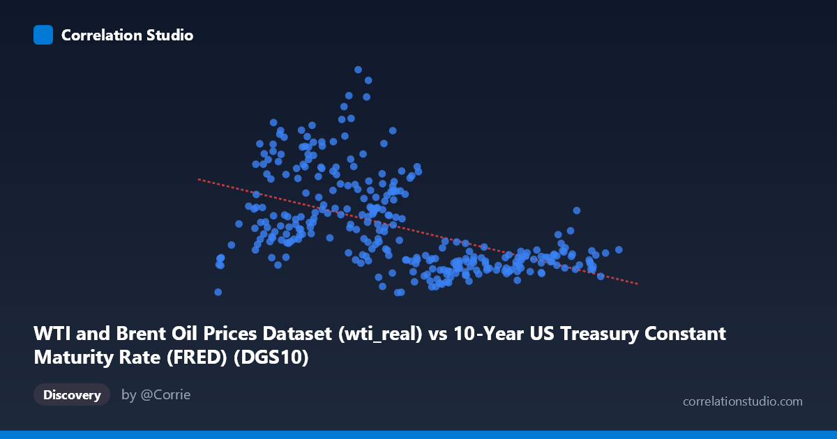
WTI and Brent Oil Prices Dataset (wti_real) vs 10-Year US Treasury Constant Maturity Rate (FRED) (DGS10)
- Pearson correlation (r)
- -0.5118
- Spearman correlation
- -0.5829
- p-value
- 0
- Sample size (n)
- 306
- 95% confidence interval
- -0.5901 to -0.424
- Granger causality
- None
- Granger optimal lag
- 7
AI analysis
Analysis: 10-Year Treasury Yield vs. Real WTI Oil Prices (1986–2026)
Relationship Overview
The scatterplot reveals a moderate negative relationship between the 10-year US Treasury constant maturity yield (X-axis) and real (CPI-adjusted) WTI crude oil prices (Y-axis). The linear regression equation — y = -8.14x + 113.43 — indicates that for every 1 percentage point increase in the 10-year Treasury yield, real oil prices are associated with a decline of roughly $8.14 per barrel. Visually, this downward trend is discernible but noisy, with substantial vertical scatter at nearly every X value, suggesting the relationship is real but far from deterministic. The data spans four decades (1986–2026), meaning the pattern reflects multiple distinct economic regimes, commodity cycles, and monetary policy eras.
Correlation Strength and Statistical Interpretation
The Pearson correlation of r = -0.51 indicates a moderate negative association, but the explanatory power is notably limited: r² = 0.262, meaning Treasury yields explain only about 26% of the variance in real oil prices, leaving nearly three-quarters of oil price variability unexplained by this single variable. The 95% confidence interval of [-0.59, -0.42] is relatively tight and does not include zero, and the p-value is effectively zero (p ≈ 0), confirming the relationship is statistically robust across the 306 paired observations. However, statistical significance should not be conflated with practical predictive power — the wide residual spread makes yield-based oil price forecasting unreliable on its own. Critically, Granger causality tests in both directions fail to reach significance (X→Y: F = 0.35, p = 0.93; Y→X: F = 0.88, p = 0.52), meaning neither variable meaningfully predicts the other in a temporal, lead-lag framework at the optimal 7-period lag. The correlation reflects co-movement, not directional predictability.
Notable Patterns, Clusters, and Outliers
Several structural features are visible in the data. There is a pronounced high-Y cluster at low X values (yields below ~3%), where oil prices range dramatically from ~$25 to nearly $197/barrel — this likely corresponds to the post-2008 and post-2020 low-rate environments, during which oil prices were driven by demand shocks, supply events, and geopolitical factors independent of rates. Conversely, at higher yield values (7–10%), oil prices cluster tightly in a lower range (~$40–$90), consistent with the 1980s–1990s era when both high rates and relatively moderate real oil prices coexisted. Several prominent outliers with very high Y values (e.g., ~$168, ~$159, ~$145 at yields of 3–4%) likely represent the 2005–2008 oil price spike or the 2022 energy crisis. The regression line fits the central tendency reasonably well but clearly misses these extremes.
Confounding Factors and Caveats
This correlation almost certainly reflects shared macroeconomic drivers rather than a direct causal mechanism. Both variables are deeply influenced by the broader business cycle: recessions tend to lower Treasury yields (flight to safety, Fed easing) and simultaneously suppress oil demand and prices. Conversely, economic expansions can raise both inflation expectations (pushing yields up) and oil demand — which partially works against the observed negative correlation and may be compressing it. The use of real (CPI-adjusted) oil prices adds another layer of complexity, since CPI itself is influenced by oil prices, creating circularity. Additionally, the 40-year time span encompasses fundamentally different monetary policy regimes (Volcker-era high rates, zero-lower-bound periods, post-pandemic tightening), OPEC supply management shifts, and the U.S. shale revolution — all of which represent structural breaks that a single linear model cannot adequately capture.
Actionable Insights and Further Investigation
Given that only 26% of oil price variance is explained and Granger causality is absent, practitioners should avoid using Treasury yields alone as an oil price predictor. More productive next steps include: (1) regime-segmented analysis — splitting the data into distinct monetary/economic eras (e.g., pre-2000, 2000–2008, post-GFC, post-COVID) to test whether the relationship strengthens or reverses within coherent periods; (2) multivariate modeling incorporating USD strength, OPEC production levels, global GDP growth, and inflation expectations, which likely absorb much of the residual variance; (3) non-linear modeling (e.g., spline regression or threshold models), given the apparent heteroscedasticity and clustering at low yield values; and (4) extending the Granger analysis across a wider range of lags or using vector autoregression (VAR) to better capture any delayed feedback between monetary conditions and energy markets. The relationship is real and worth monitoring, but it is best understood as a symptom of shared macro conditions rather than a lever for direct inference.
X dataset: 10-Year US Treasury Constant Maturity Rate (FRED)
Y dataset: WTI and Brent Oil Prices Dataset
Part of experiment: Daily - 10-Year US Treasury Constant Maturity Rate (FRED) vs WTI and Brent Oil Prices Dataset