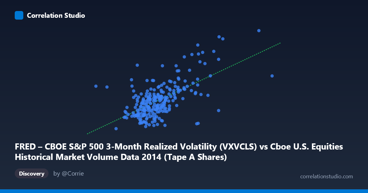
FRED – CBOE S&P 500 3-Month Realized Volatility (VXVCLS) vs Cboe U.S. Equities Historical Market Volume Data 2014 (Tape A Shares)
- Pearson correlation (r)
- 0.617
- Spearman correlation
- 0.538
- p-value
- 0
- Sample size (n)
- 252
- 95% confidence interval
- 0.5341 to 0.6881
- Granger causality
- None
- Granger optimal lag
- 1
AI analysis
Analysis: CBOE S&P 500 3-Month Realized Volatility vs. Tape A Shares Volume (2014)
Relationship Overview
The scatterplot reveals a moderate positive relationship between CBOE S&P 500 3-month realized volatility (VXVCLS) and Tape A share volume for U.S. equities in 2014. As trading volume increases, realized volatility tends to rise in tandem — a relationship that aligns well with established market microstructure theory, where elevated trading activity is frequently associated with periods of price uncertainty and heightened investor reactivity. The linear regression equation (y = 2.70×10⁻⁸x + 9.37) confirms this positive slope, though the intercept suggests a baseline volatility level even when volume is relatively subdued.
Correlation Strength and Statistical Significance
The correlation coefficient of r = 0.617 indicates a moderately strong positive association, but the more telling figure is r² = 0.381, meaning that only about 38% of the variance in volatility is explained by trading volume. The remaining 62% is attributable to other factors not captured here. The 95% confidence interval of [0.534, 0.689] is relatively narrow and does not include zero, and the p-value of essentially 0 confirms this is not a chance finding across the 252 paired observations drawn from a population of 3,686. That said, statistical significance here should not be conflated with practical predictive power — the unexplained majority of variance is a meaningful limitation. Critically, Granger causality testing finds no significant predictive direction in either direction (X→Y: F=2.37, p=0.125; Y→X: F=0.65, p=0.420), meaning that neither variable reliably predicts the other at a one-period lag. This suggests the relationship is contemporaneous rather than lead-lag, likely driven by shared responses to common market events rather than one variable driving the other sequentially.
Notable Patterns, Clusters, and Outliers
Several structural features are visible in the data. The bulk of observations cluster in a relatively tight band at lower volume levels (roughly 150M–270M shares), where volatility spans a wide range (approximately 12–19), suggesting that at moderate volumes, other factors dominate volatility dynamics. However, there is a visually distinct upper-right cluster of high-volume, high-volatility observations (notably points near 350M–370M shares with volatility of 22–23), which likely correspond to specific stress episodes in late 2014 — potentially October's sharp equity selloff. There also appear to be low-volatility outliers at high volume (e.g., ~311M shares at ~12.87 volatility), which are structurally inconsistent with the general trend and may represent end-of-year or expiration-driven volume spikes that did not coincide with genuine price stress. One point at a very low X value (~101M shares, ~17.26 volatility) also sits notably off the main cluster, suggesting that very low-volume days are not necessarily calm ones.
Confounding Factors and Caveats
Several important caveats apply. First, both variables are likely jointly driven by exogenous macro or geopolitical shocks — events like Federal Reserve announcements, geopolitical stress (Russia/Ukraine tensions in 2014), or oil price dislocations would simultaneously elevate both volume and volatility, manufacturing correlation without direct causation. Second, the three-month realized volatility measure is backward-looking and smoothed, meaning it may lag intraday or single-session volume spikes, which could dampen the observed relationship. Third, Tape A shares represent only NYSE-listed securities, while VXVCLS reflects the broader S&P 500 universe — this cross-dataset mismatch introduces measurement noise. Finally, 2014 was a relatively low-volatility year by historical standards, so the dynamic captured here may not generalize to crisis periods where both variables behave more non-linearly.
Actionable Insights and Further Investigation
Practitioners could explore several natural extensions. Given the lack of Granger causality, intraday or same-day analysis may be more informative than lagged models — the relationship appears to operate on a contemporaneous basis, suggesting real-time regime monitoring rather than predictive signaling is the appropriate application. It would be valuable to segment the data by market regime (e.g., pre- and post-October 2014 stress period) to test whether the correlation is driven disproportionately by a handful of high-stress episodes. Additionally, adding control variables such as VIX levels, Fed announcement dates, or options expiration calendars could help disentangle the shared-shock explanation. Finally, extending this analysis across multiple years would clarify whether the 2014 r=0.617 is representative of a structural relationship or an artifact of that year's specific volatility clustering.
X dataset: Cboe U.S. Equities Historical Market Volume Data 2014
Y dataset: FRED – CBOE S&P 500 3-Month Realized Volatility
Part of experiment: Daily - Cboe U.S. Equities Historical Market Volume Data 2014 vs FRED – CBOE S&P 500 3-Month Realized Volatility