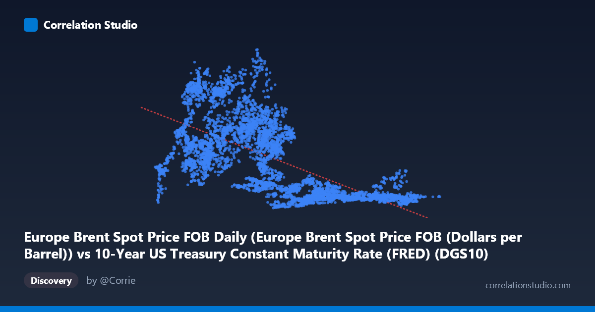
Europe Brent Spot Price FOB Daily (Europe Brent Spot Price FOB (Dollars per Barrel)) vs 10-Year US Treasury Constant Maturity Rate (FRED) (DGS10)
- Pearson correlation (r)
- -0.657
- Spearman correlation
- -0.709
- p-value
- 0
- Sample size (n)
- 9642
- 95% confidence interval
- -0.6682 to -0.6455
- Granger causality
- None
- Granger optimal lag
- 1
AI analysis
Analysis: Europe Brent Crude Oil Price vs. 10-Year US Treasury Yield
Relationship Overview The scatterplot reveals a negative relationship between Europe Brent crude oil spot prices (X-axis) and the 10-year US Treasury constant maturity rate (Y-axis), captured over nearly four decades (1987–2026). The linear regression equation (y = -9.68x + 95.13) suggests that for every $1/barrel increase in Brent crude, the 10-year Treasury yield tends to decrease by approximately 0.97 percentage points — a counterintuitive direction that immediately warrants careful interpretation. The sample points illustrate considerable scatter, with low oil prices (X ~1.3–2.5) frequently pairing with high Treasury yields (Y ~40–125), while higher oil prices (X ~7–10) cluster tightly at low yield values (~15–20).
Correlation Strength and Statistical Significance The Pearson correlation of r = -0.657 indicates a moderate-to-strong negative association, with r² = 0.432 meaning that approximately 43% of the variance in Treasury yields is statistically explained by oil prices in this paired dataset. The 95% confidence interval of [-0.668, -0.646] is exceptionally narrow given the large sample (n = 9,642), and the p-value of effectively zero confirms this relationship is not attributable to chance. However, Granger causality tests tell a critically different story: neither direction (X→Y: F=0.52, p=0.47; Y→X: F=1.34, p=0.25) reaches significance at any conventional threshold. This means that while a strong contemporaneous correlation exists, neither variable reliably predicts the other temporally — a crucial distinction separating statistical association from causal or predictive utility.
Notable Patterns, Clusters, and Non-Linearity The sample points reveal two visually distinct clusters rather than a smooth linear trend. A dense cluster sits at high X values (6–10) with uniformly low Y values (~10–25), while a more dispersed cluster occupies low X values (1–4) with widely ranging Y values (~20–125). This bimodal structure strongly hints at non-linearity — potentially a hyperbolic or inverse relationship rather than a purely linear one. Several notable outliers appear at low oil prices with extremely high Treasury yields (~119–125 range), likely corresponding to the early 1987–1990 period when both interest rates and oil dynamics were distinctly different. The variance in Y expands dramatically as X decreases, suggesting heteroscedasticity that undermines standard linear regression assumptions.
Confounding Factors and Interpretive Caveats The most significant caveat is that both variables are strongly time-dependent, evolving through completely different macroeconomic regimes over 39 years. Treasury yields were structurally declining from ~9% in the late 1980s through the 2010s (secular rate decline), while oil prices underwent multiple independent boom-bust cycles (Gulf War, 2008 spike, 2014–2016 collapse, COVID crash). The apparent negative correlation likely reflects a spurious temporal coincidence: high interest rate eras preceded the widespread commercialization of oil futures pricing, while the shale revolution and post-2008 monetary policy independently drove both oil volatility and near-zero yields. The axes appear to be swapped from their natural roles — oil price is plotted on X while Treasury yield is on Y, and the dataset labels confirm this inversion — which should be corrected before drawing directional conclusions.
Actionable Insights and Further Investigation Given the absence of Granger causality and the strong temporal confounding, practitioners should avoid using this correlation for predictive modeling without substantial controls. Recommended next steps include: (1) regime-segmented analysis — breaking the dataset into distinct macroeconomic periods (pre/post-2008, pre/post-shale revolution) to test whether the correlation holds within regimes or only emerges from cross-regime level differences; (2) cointegration testing to determine whether any long-run equilibrium relationship exists beyond spurious correlation; (3) multivariate modeling incorporating inflation (CPI/PCE), Federal Reserve policy rate, and USD index as confounders; (4) applying non-linear regression (inverse or log-log) to better capture the apparent hyperbolic structure. The relationship is statistically robust but economically fragile, and should be treated as a descriptive historical artifact rather than an actionable signal.
X dataset: 10-Year US Treasury Constant Maturity Rate (FRED)
Y dataset: Europe Brent Spot Price FOB Daily
Part of experiment: Daily - 10-Year US Treasury Constant Maturity Rate (FRED) vs Europe Brent Spot Price FOB Daily