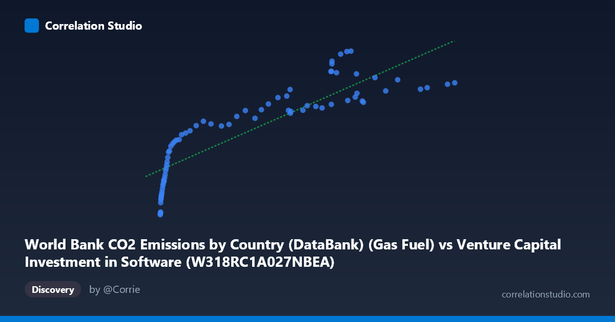
World Bank CO2 Emissions by Country (DataBank) (Gas Fuel) vs Venture Capital Investment in Software (W318RC1A027NBEA)
- Pearson correlation (r)
- 0.8612
- Spearman correlation
- 0.9511
- p-value
- 0
- Sample size (n)
- 75
- 95% confidence interval
- 0.7883 to 0.9103
- Granger causality
- None
- Granger optimal lag
- 10
AI analysis
Scatterplot Analysis: Gas Fuel CO2 Emissions vs. Venture Capital Investment in Software
Relationship Overview
The scatterplot reveals a positive, moderately strong relationship between gas fuel CO2 emissions and venture capital investment in software over the period 1946–2020. As gas fuel emissions increase, VC software investment tends to rise as well, following a broadly linear trend captured by the regression equation y = 27.46x + 5,228.63. However, the relationship is not uniformly tight across the full range of X values — the data exhibits notably wider vertical spread at higher emission levels (roughly X 200), suggesting that while the general trend holds, the predictive precision weakens considerably at the upper end of the distribution. The wide X range (0.85 to 466.42) and Y range (854.77 to 16,992.26) reflect substantial temporal growth across the 74-year coverage window, likely tracking post-war industrialization and the modern tech economy's simultaneous expansion.
Correlation Strength, Direction, and Statistical Significance
The Pearson correlation of r = 0.8612 indicates a strong positive association, and the R² of 0.7417 means approximately 74.2% of the variance in VC software investment is statistically explained by gas fuel CO2 emissions within this linear model. That leaves roughly 26% of variance attributable to other factors. The 95% confidence interval for r [0.7883, 0.9103] is relatively narrow and lies entirely above zero, reinforcing that the association is robust and not a statistical artifact. The p-value of effectively zero confirms the correlation is highly statistically significant at any conventional threshold. Critically, however, the Granger causality results undercut any causal interpretation entirely: neither X→Y (F = 0.304, p = 0.976) nor Y→X (F = 0.572, p = 0.828) reaches significance at even the most lenient threshold, even with an optimal lag of 10 periods. This means neither variable temporally predicts the other, strongly suggesting the correlation is driven by a shared confounding trend rather than any directional causal mechanism.
Notable Patterns, Clusters, and Outliers
The data cluster into two visually distinct regions. The first is a dense, steeply rising cluster at low X values (0–50), where Y spans roughly 854 to 10,000 — this steep early rise reflects rapid proportional growth in both variables from modest baselines, likely corresponding to the post-WWII through 1980s era. The second is a diffuse cloud at higher X values (200–470), where Y ranges widely from approximately 10,000 to 17,000 despite relatively small changes in X, suggesting diminishing marginal returns or a plateau dynamic. Several points warrant attention as potential outliers: the cluster around X ≈ 270–310 shows unusually high Y values (14,983–16,992), including the maximum Y observation (302.31, 16,992.26), pulling the regression line upward. Conversely, the lowest observations (X < 5, Y < 3,500) are tightly grouped and well-fitted by the linear model. This heteroscedasticity — variance in Y expanding with X — suggests a logarithmic or power transformation of X might produce a better-fitting model.
Confounding Factors and Interpretive Caveats
The most significant caveat here is that both variables are almost certainly co-trending with time. From 1946 to 2020, both global CO2 emissions from gas fuel and US venture capital investment in software grew enormously for entirely independent structural reasons — one driven by energy demand and fossil fuel infrastructure, the other by the emergence of the digital economy. When two time series share a common upward trend, spurious correlations with high r and R² values are virtually guaranteed, regardless of any real-world relationship between the variables. The failed Granger causality tests confirm this interpretation. Additionally, the dataset label mismatch is notable — the X-axis column label references "Venture Capital Investment in Software" but the source is described as "World Bank CO2 Emissions," and vice versa for Y, suggesting possible metadata confusion that should be audited before drawing any conclusions. The 74-year time span also conflates very different economic and geopolitical regimes, making stationarity assumptions for any predictive model highly questionable.
Actionable Insights and Further Investigation
Given the strong evidence of spurious correlation driven by shared temporal trends, the most important next step is to detrend both series — for example, by differencing, applying Hodrick-Prescott filtering, or analyzing year-over-year growth rates — and then re-evaluate the correlation on the residuals. If the correlation disappears after detrending, the relationship is confirmed as spurious. Analysts should also verify and correct the dataset metadata labels, as the apparent column-to-dataset mismatch raises data integrity concerns. Further investigation could explore whether a nonlinear model (logarithmic or piecewise) better captures the steep early rise and plateau at high X values, which the linear R² of 74% partially masks. Finally, introducing structural break analysis around key periods (e.g., the 1970s oil crisis, the 1990s dot-com boom, the 2008 financial crisis) could reveal whether the apparent relationship is driven by a specific sub-period rather than a consistent mechanism across the full 74-year window.
X dataset: Venture Capital Investment in Software
Y dataset: World Bank CO2 Emissions by Country (DataBank)
Part of experiment: Yearly - Venture Capital Investment in Software vs World Bank CO2 Emissions by Country (DataBank)