Bitcoin Market Capitalization Time Series (Total Supply) vs CryptoDataDownload – Binance BTC/USDT Daily OHLCV (High)
- Pearson correlation (r)
- -0.6997
- Spearman correlation
- -0.6415
- p-value
- 0.000099
- Sample size (n)
- 25
- 95% confidence interval
- -0.8577 to -0.4209
- Granger causality
- None
- Granger optimal lag
- 6
AI analysis
Scatterplot Analysis: BTC Market Cap vs. BTC High Price
1. Overview of the Relationship
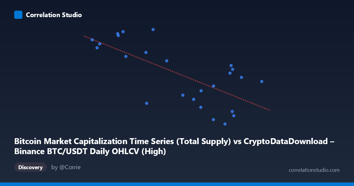
The scatterplot displays 25 paired observations between a Bitcoin market capitalization proxy (X) and the daily "High" price series (Y) over a roughly one-month window (March 29 – April 22, 2024). Visually, the points form a downward-sloping cloud: as X increases, Y tends to decrease, but the scatter is fairly wide, with no tight linear band. The relationship is discernible but noisy rather than a clean, deterministic line.
2. Strength, Direction, and Statistical Confidence
The correlation coefficient (r = -0.70) indicates a moderate-to-strong negative relationship. Squaring this (R² = 0.49) shows that only about 49% of the variance in Y is explained by X, leaving roughly half of the variability attributable to other factors or noise. The 95% confidence interval for r [-0.858, -0.421] is fairly wide, reflecting the small sample size (n=25), but it does exclude zero, and the p-value (9.9e-05) is highly significant — so we can be confident a real negative association exists, even though its precise strength is uncertain. Importantly, the Granger causality tests show no significant predictive direction in either direction (X→Y p=0.315; Y→X p=0.385). This means that despite the contemporaneous negative correlation, neither series reliably leads or forecasts the other over the tested lag structure — the relationship appears more coincidental/contemporaneous than causal or sequential.
3. Patterns, Clusters, and Outliers
The data does not show obvious clustering into distinct regimes, but there is a visible split: lower X values (~64,000–66,000) tend to pair with higher Y values (~19,682,000–19,688,800), while higher X values (~70,000–72,800) pair with lower Y values (~19,668,000–19,680,000). The point at (72797.99, 19677331.25) is somewhat of a mild outlier — it has the highest X value but a mid-range Y, slightly breaking the downward trend. No strong curvature or non-linear pattern (e.g., U-shape) is apparent; a linear fit seems like a reasonable first-order approximation, though the residual scatter suggests the true relationship may be more complex or influenced by additional variables.
4. Caveats and Potential Confounders
Several caveats limit interpretation. First, the sample size (n=25) is small, making the correlation estimate sensitive to individual points and the CI wide. Second, this is a short time window (~3.5 weeks), so the observed relationship may reflect a temporary market regime rather than a structural one. Third, and critically, the two variables are definitionally related — market capitalization is typically calculated as price × circulating supply, so "Market Cap" and "High price" are not fully independent measures; their negative correlation here may partly reflect how circulating supply or the specific computation methodology moved inversely to price during this period, rather than an economically meaningful independent relationship. Finally, both series are drawn from BTC/USDT data possibly subject to exchange-specific quirks (e.g., Binance-specific liquidity or reporting artifacts) that may not generalize.
5. Suggestions for Further Investigation
Given the ambiguous causality and moderate R², further analysis should: (1) extend the time window to increase sample size and test whether the negative correlation persists or reverses in different market regimes (bull vs. bear); (2) investigate the supply-side component driving market cap independently of price, to clarify whether the negative correlation is a mechanical artifact of decreasing supply growth during price rallies; (3) test alternative lag structures or non-linear causality models (e.g., nonlinear Granger, transfer entropy) given the inconclusive linear Granger results; and (4) incorporate additional variables (trading volume, macro indicators, on-chain flows) to determine if a third factor is driving both series simultaneously, which would explain the correlation without direct causality.
X dataset: CryptoDataDownload – Binance BTC/USDT Daily OHLCV
Y dataset: Bitcoin Market Capitalization Time Series
Part of experiment: Bitcoin - CryptoDataDownload – Binance BTC/USDT Daily OHLCV vs Bitcoin Market Capitalization Time Series