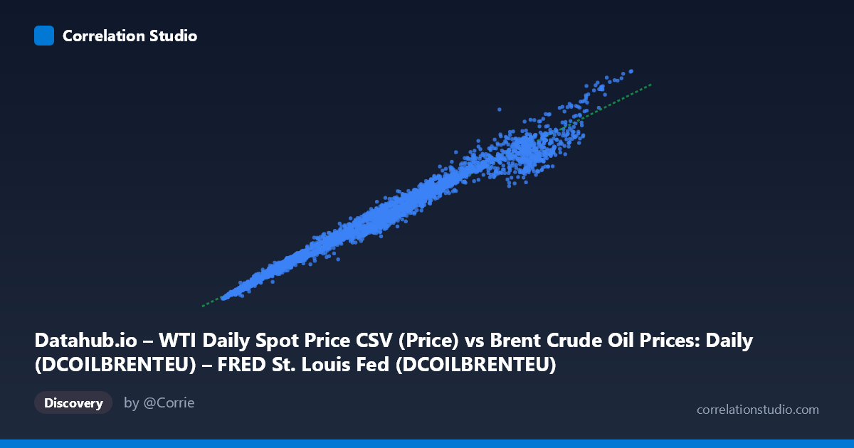
Datahub.io – WTI Daily Spot Price CSV (Price) vs Brent Crude Oil Prices: Daily (DCOILBRENTEU) – FRED St. Louis Fed (DCOILBRENTEU)
- Pearson correlation (r)
- 0.9911
- Spearman correlation
- 0.995
- p-value
- 0
- Sample size (n)
- 9718
- 95% confidence interval
- 0.9907 to 0.9914
- Granger causality
- None
- Granger optimal lag
- 1
AI analysis
Analysis: Brent Crude (Datahub.io) vs. WTI Crude (FRED)
1. Overall Relationship The scatterplot reveals an exceptionally tight, nearly linear relationship between the Datahub.io WTI Daily Spot Price and the FRED Brent Crude Daily price. Points cluster very closely along a straight diagonal line from the lower-left (prices near ~$10–15/barrel) to the upper-right (prices approaching ~$140–145/barrel), visually confirming what is essentially a near-perfect positive linear association across nearly four decades of daily pricing data. This is unsurprising given that both series track global crude oil markets, but the tightness of the fit is still striking.
2. Correlation Strength and Statistical Framing The Pearson correlation of r = 0.9911 is extraordinarily high, and the R² of 0.9823 means that approximately 98.2% of the variance in WTI prices is statistically explained by Brent prices (or vice versa), leaving only ~1.8% unexplained by the linear model. The 95% confidence interval of [0.9907, 0.9914] is vanishingly narrow, reflecting the large paired sample size (n = 9,718), and the p-value of effectively 0 makes any doubt about the reality of this correlation statistically negligible. The regression equation y = 0.8858x + 4.13 is telling: the slope below 1.0 and positive intercept indicate that WTI prices are systematically slightly lower than Brent prices, consistent with the well-known historical Brent premium, particularly pronounced since ~2011. However, the Granger causality tests are non-significant in both directions (X→Y: F = 1.06, p = 0.30; Y→X: F = 0.94, p = 0.33), meaning neither series reliably predicts the other at a one-period lag beyond what each already predicts about itself. This is consistent with two series that are driven by the same underlying global supply-and-demand forces simultaneously, rather than one leading the other.
3. Notable Patterns, Clusters, and Outliers Several structural features are visible in the sample points and implied by the data distribution. There is a heavy concentration of points in the $10–$30 range (lower-left cluster), reflecting the extended periods of low oil prices in the late 1980s–1990s and post-2015 era. A secondary dense cluster appears around $40–$80, corresponding to the 2000s run-up and post-2008 recovery. The extreme upper-right points (~$135–$145) correspond to the 2008 price spike, which represents a relative outlier in magnitude but still falls on the regression line, suggesting the linear relationship held even under extreme market stress. A few points show slightly wider Brent-WTI spreads (e.g., 109.46 vs. 99.47; 113.21 vs. 100.32), likely reflecting the 2011–2013 period when U.S. pipeline infrastructure constraints caused WTI to trade at an unusual discount to Brent.
4. Caveats and Confounding Factors The most important interpretive caveat is that this correlation is largely tautological: both variables are global crude oil benchmark prices tracking the same underlying commodity market, so high correlation is structurally expected rather than analytically surprising. The regression slope (~0.886) reflects the historically variable Brent-WTI spread, which is not constant — it has ranged from near-parity to over $20/barrel depending on U.S. midcontinent logistics, export policy, and geopolitical context. This means the linear model will systematically misbehave during regime-change periods. Additionally, the two datasets come from different data providers (Datahub.io vs. FRED), raising the possibility of minor differences in data cleaning, date alignment, or revision policies that could introduce small artificial discrepancies. The non-significant Granger result should also be interpreted cautiously: at a daily lag, both markets respond nearly simultaneously to news, so the absence of directional predictability is expected and does not mean the series are economically independent.
5. Actionable Insights and Further Investigation The near-perfect correlation confirms these two datasets are effectively interchangeable for most analytical purposes, but the systematic slope-below-1 and nonzero intercept suggest a spread model would be more precise than a simple ratio. Analysts should investigate the time-varying Brent-WTI spread as a separate signal — plotting residuals from this regression over time would likely reveal the 2011–2013 infrastructure disruption period as a structural break worth modeling explicitly. For predictive modeling, adding spread-driving covariates (Cushing inventory levels, U.S. export volumes, pipeline capacity) could explain the residual 1.8% variance. It would also be worth testing nonlinear or piecewise regression to check whether the relationship changes across price regimes (low < $40, medium $40–$80, high $80). Finally, the dataset's extension to 2026 should be carefully validated, as future-dated observations likely reflect futures prices or forecasts rather than spot prices, which could introduce systematic bias into correlation estimates.
X dataset: Brent Crude Oil Prices: Daily (DCOILBRENTEU) – FRED St. Louis Fed
Y dataset: Datahub.io – WTI Daily Spot Price CSV
Part of experiment: Daily - Brent Crude Oil Prices: Daily (DCOILBRENTEU) – FRED St. Louis Fed vs Datahub.io – WTI Daily Spot Price CSV