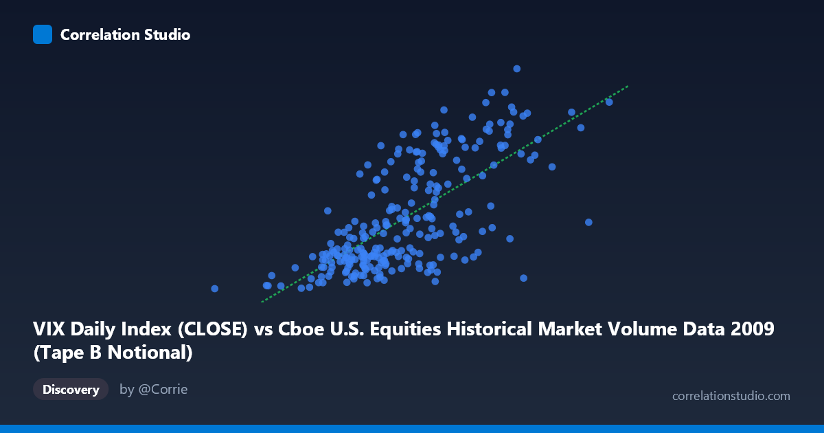
VIX Daily Index (CLOSE) vs Cboe U.S. Equities Historical Market Volume Data 2009 (Tape B Notional)

Pearson correlation (r): 0.693
Spearman correlation: 0.6837
p-value: 0
Sample size (n): 252
95% confidence interval: 0.6228 to 0.7522
Granger causality: None
Granger optimal lag: 1

AI analysis

Scatterplot Analysis: VIX Daily Index vs. Tape B Notional Volume (2009)

Overall Relationship

The scatterplot reveals a moderately positive relationship between the VIX Daily Index close values and Tape B Notional trading volume across 2009. As VIX levels rise, Tape B Notional volume tends to increase, which is intuitively consistent with the well-established market phenomenon whereby heightened volatility drives elevated trading activity. The linear regression equation (y = 4.80×10⁻⁹x + 6.14) confirms this upward slope, though the wide dispersion of points around the regression line makes clear that this is far from a deterministic relationship. The data spans a full calendar year (January–December 2009), capturing the tail end of the global financial crisis and the subsequent market recovery — a period of historically exceptional volatility dynamics.

Correlation Strength and Statistical Significance

The Pearson correlation of r = 0.693 indicates a moderate-to-strong positive association, but the more practically meaningful statistic is r² = 0.4803, meaning that VIX levels explain approximately 48% of the variance in Tape B Notional volume. While this is substantial, it equally implies that roughly 52% of the variance remains unexplained by VIX alone, underscoring the need for additional predictive variables. The 95% confidence interval [0.623, 0.752] is relatively tight and does not approach zero, and the p-value of effectively 0 across a paired sample of n = 252 (drawn from N = 3,232) confirms that this correlation is highly unlikely to be a statistical artifact. However, the Granger causality results tell a more cautionary story: neither direction (X→Y nor Y→X) reaches significance (F = 0.043, p = 0.837 for VIX predicting volume; F = 0.360, p = 0.549 for volume predicting VIX), indicating that neither variable temporally predicts the other at a one-period lag. This means the correlation is contemporaneous rather than predictive — VIX and Tape B volume move together, but knowing yesterday's VIX does not help forecast today's volume, and vice versa.

Notable Patterns, Clusters, and Outliers

Several structural features stand out in the sample points. There appears to be a bimodal clustering tendency: a dense lower cluster concentrated roughly between VIX values of 19–27 and lower notional volumes, and a more dispersed upper cluster at higher VIX readings (40–56) with elevated volume figures. This bifurcation likely reflects the market's transition during 2009 from crisis-era extreme volatility in early months to a calmer regime as the year progressed. Notable outliers include points such as (7,068,706,762, 52.62) and (7,346,093,685, 52.65), which represent episodes of simultaneously very high VIX and very high volume — consistent with acute stress events. Conversely, some points exhibit high VIX with relatively modest volume (e.g., 6,788,289,545 at VIX 25.61), suggesting that the relationship is heteroscedastic: variance in volume appears to fan outward as VIX increases, which violates a key assumption of simple linear regression.

Confounding Factors and Interpretive Caveats

Several important caveats apply. First, 2009 is a highly anomalous year — the S&P 500 bottomed in March and staged a dramatic recovery, meaning that both VIX levels and volume behavior were driven by an overarching macro crisis narrative rather than typical market conditions. Any correlation derived from this period may not generalize to normal market environments. Second, Tape B Notional specifically covers NYSE American (AMEX) and regional exchange-listed securities, which may respond differently to volatility than the broader market. Third, institutional trading strategies, algorithmic volume responses, and circuit-breaker mechanisms during the crisis period could all drive both variables simultaneously without a direct causal link — classic common-cause confounding. Fourth, the heteroscedasticity noted above means the linear model's predictive error is systematically larger at high VIX values, reducing practical utility precisely when accurate forecasting matters most.

Actionable Insights and Further Investigation

Practitioners should treat this correlation as a useful contemporaneous signal rather than a predictive tool, given the absence of Granger causality. For further investigation, it would be valuable to: (1) segment the analysis by quarter to test whether the correlation is driven predominantly by the crisis months (Q1) versus the recovery (Q2–Q4); (2) apply a log transformation to the notional volume variable to address heteroscedasticity and potentially improve model fit; (3) introduce additional covariates such as S&P 500 returns, bid-ask spreads, or Fed intervention dates to better isolate the VIX-volume relationship; and (4) replicate this analysis across multiple years to determine whether r ≈ 0.69 is a stable structural feature or a crisis-specific artifact. A threshold or regime-switching model may ultimately outperform linear regression, given the apparent clustering behavior visible in the data.

X dataset: Cboe U.S. Equities Historical Market Volume Data 2009

Y dataset: VIX Daily Index

Part of experiment: Daily - Cboe U.S. Equities Historical Market Volume Data 2009 vs VIX Daily Index