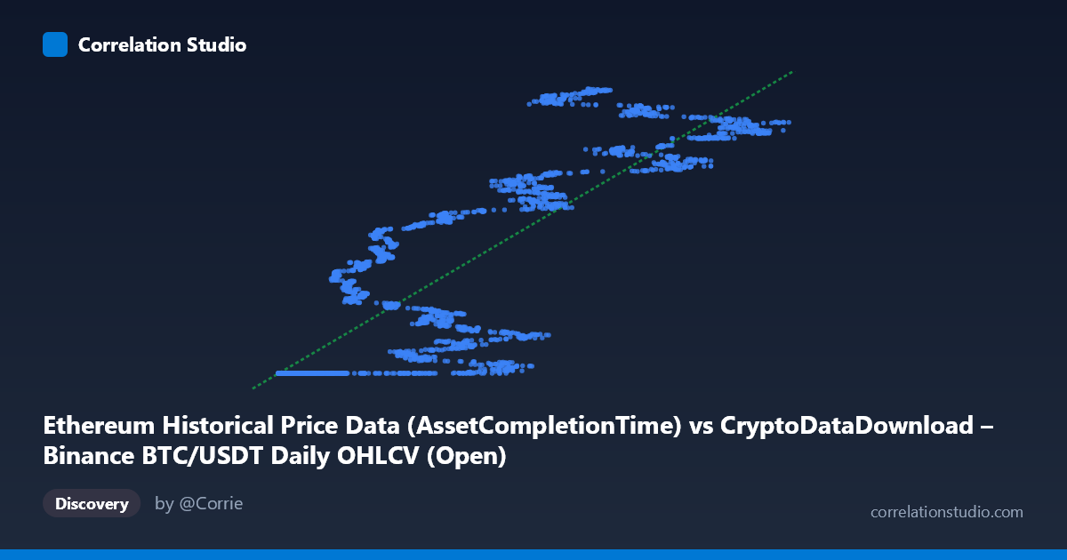
Ethereum Historical Price Data (AssetCompletionTime) vs CryptoDataDownload – Binance BTC/USDT Daily OHLCV (Open)
- Pearson correlation (r)
- 0.8524
- Spearman correlation
- 0.8876
- p-value
- 0
- Sample size (n)
- 3191
- 95% confidence interval
- 0.8426 to 0.8616
- Granger causality
- None
- Granger optimal lag
- 10
- Time coverage
- 2017-08-17 to 2026-05-20
AI analysis
Analysis: Ethereum "Completion Time" Metric vs. BTC/USDT Opening Price
1. What the Visualization Reveals
The scatterplot shows a strong positive, non-linear relationship between the X variable (labeled as an Ethereum-related timestamp/completion metric) and Y (BTC/USDT opening price). Notably, the sample data reveals a striking pattern: for X values below roughly 20,000, Y is essentially pinned to a narrow band near 1,614,335,000–1,614,335,700 — suspiciously uniform given the enormous range of Y overall (1.61B to 1.78B). Once X exceeds ~20,000–25,000, Y begins climbing steeply and continues rising with increasing X, though with substantial scatter. This suggests a threshold or floor effect rather than a purely linear relationship.
2. Strength, Direction, and Statistical Meaning
The Pearson correlation (r = 0.852) and R² (0.727) indicate a strong positive association, with X explaining about 73% of the variance in Y — a substantial but not complete relationship, leaving ~27% of variance driven by other factors or noise. The tight 95% CI [0.843, 0.862] and p-value effectively at 0 confirm this correlation is highly statistically robust and not a artifact of sampling noise, given the large N (~3,191). However, statistical significance here reflects sample size, not causal strength or model correctness — especially since the underlying relationship appears non-linear (see Section 3), meaning the linear R² likely understates true explanatory power in the fitted regions but overstates it in the flat "floor" region.
Critically, the Granger causality tests show no significant predictive direction in either direction (X→Y: p=0.34; Y→X: p=0.15). This means neither series reliably predicts future values of the other based on past values — the strong contemporaneous correlation is not accompanied by evidence of temporal lead-lag dynamics. This is common in time series that share a common trend or are both driven by an external factor (e.g., overall crypto market cycles) rather than one causing the other.
3. Notable Patterns and Outliers
The most conspicuous feature is the flat "floor" cluster at low X values (~3,000–20,000), where Y remains locked near 1,614,335,000 regardless of X — this looks less like organic price data and more like a data artifact, placeholder value, or a period of extremely low/frozen pricing (possibly early exchange history or a data quality issue in the source table). Above this threshold, the relationship becomes much more dynamic, with Y ranging widely (up to 1.78B) for X values from 20,000–125,000, and increasing scatter/heteroscedasticity at higher X. This fan-shaped spread at higher X values suggests variance is not constant across the range (violating a linear regression assumption), and a piecewise or logarithmic model may fit better than the straight line reported.
4. Confounding Factors and Caveats
Both variables are derived from BTC/USDT OHLCV data by description overlap (the "X" label mentions Ethereum completion time, but the dataset descriptions reference the same BTC/USDT source for both axes) — this raises concern about variable mislabeling or metadata inconsistency, which should be verified before drawing conclusions. Additionally, since both series likely reflect long-term crypto market trends (2017–2026), the correlation may be driven by a shared macro trend (broad bull market appreciation) rather than any direct mechanistic link — classic time-series confounding. The flat floor segment also suggests possible data entry errors, missing-value imputation, or an inactive trading period that should be excluded or investigated before modeling.
5. Suggestions for Further Investigation
1. Clarify variable definitions — confirm what "X" (Ethereum Historical Price Data - AssetCompletionTime) actually represents, as the label and flat segment suggest it may be a timestamp/index rather than a price. 2. Segment the analysis — separately model the flat low-X region and the rising high-X region; a piecewise regression or log/power transformation likely fits better than a single linear model. 3. Detrend both series (e.g., using returns or first differences) before assessing correlation/causality to rule out spurious correlation from shared upward market trends. 4. Investigate the flat cluster directly — check raw data for that period to confirm it's not a placeholder or stale-price artifact. 5. Given the null Granger result, avoid using one series to forecast the other in a trading context; instead, explore whether both are driven by a common exogenous factor (e.g., overall crypto market cap, BTC dominance).
X dataset: CryptoDataDownload – Binance BTC/USDT Daily OHLCV
Y dataset: Ethereum Historical Price Data
Part of experiment: Bitcoin - CryptoDataDownload – Binance BTC/USDT Daily OHLCV vs Ethereum Historical Price Data