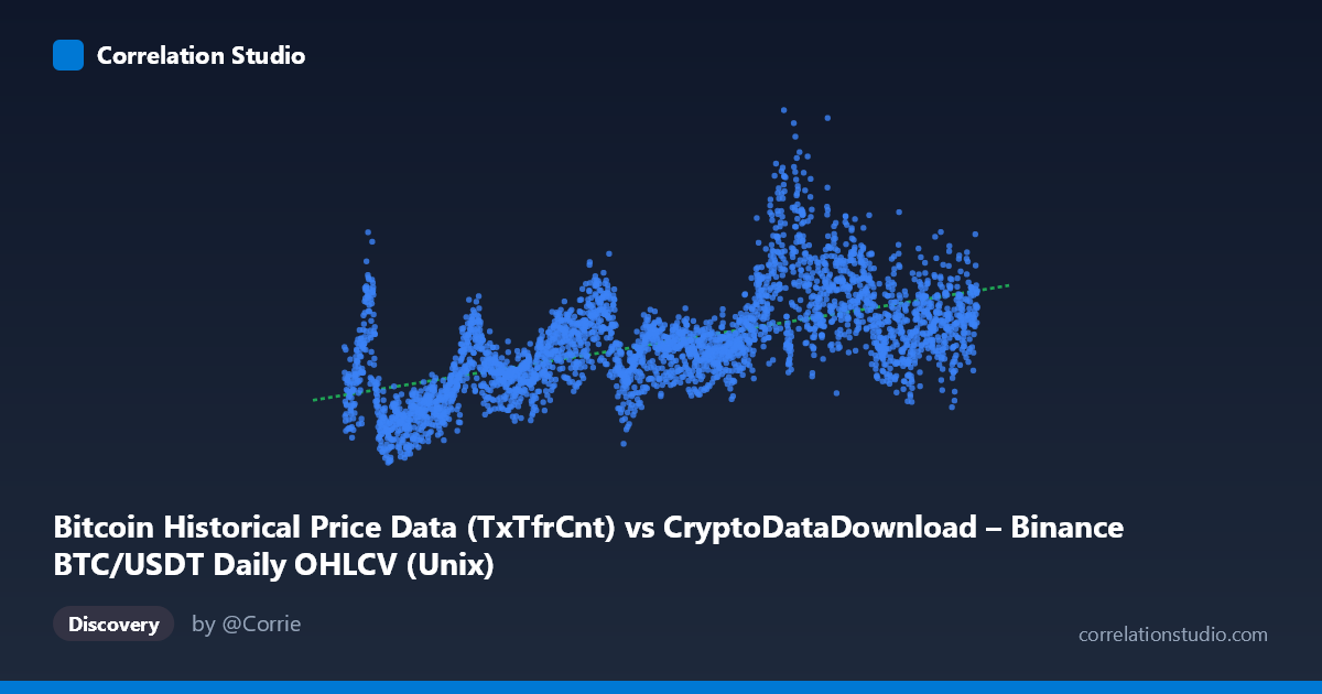
Bitcoin Historical Price Data (TxTfrCnt) vs CryptoDataDownload – Binance BTC/USDT Daily OHLCV (Unix)
- Pearson correlation (r)
- 0.6
- Spearman correlation
- 0.6278
- p-value
- 0
- Sample size (n)
- 3191
- 95% confidence interval
- 0.5774 to 0.6218
- Granger causality
- None
- Granger optimal lag
- 10
- Time coverage
- 2017-08-17 to 2026-05-20
AI analysis
Analysis of Bitcoin Time Series vs. Transaction Count Relationship
1. What the Visualization Reveals
This scatterplot examines the relationship between a time variable (X-axis, spanning 2017–2026, likely representing timestamps from the OHLCV dataset) and Y-axis values ranging from ~365K to ~1.68M (labeled as transaction count, TxTfrCnt). Despite the axis labels appearing somewhat swapped in the metadata, the core finding is that Y-values generally trend upward over the ~9-year period, though with substantial scatter and volatility, particularly in the middle years (2020–2024) where values spike well above the general trend (e.g., readings near 1.1–1.4M against a mean of ~813K).
2. Strength, Direction, and Statistical Confidence
The correlation coefficient (r = 0.60) indicates a moderate positive relationship, with the linear model explaining only 36% of the variance (R² = 0.36) in Y. This means nearly two-thirds of the variability in Y is driven by factors other than the simple linear time trend — the relationship is real but far from deterministic. The 95% confidence interval [0.577, 0.622] is tight, and the p-value ≈ 0 confirms this correlation is highly statistically significant and not due to chance, aided by the large sample size (n=3,191). However, statistical significance should not be conflated with strong predictive power — R² of 0.36 leaves considerable unexplained variance. Critically, the Granger causality tests show no significant predictive direction in either direction (X→Y: p=0.08; Y→X: p=0.75). This suggests that while the two series are correlated and co-trend over time, neither temporally leads the other in a statistically robust way — the relationship may be driven by a shared underlying trend (e.g., both increasing due to Bitcoin network growth/adoption over years) rather than one causing fluctuations in the other.
3. Notable Patterns and Outliers
The data show a clear upward secular trend punctuated by high-variance clusters. Early years (2017–2019) cluster at lower Y-values (400K–700K), consistent with early Bitcoin network activity. A pronounced volatility regime emerges around 2020–2021 and again 2023–2024, with values spiking to 1.1M–1.68M — likely corresponding to periods of heightened network usage, bull market activity, or congestion events. Some sample points show dramatic short-term jumps (e.g., 1,383,459 on one date followed by much lower values on nearby dates), suggesting the series is not smoothly trending but subject to sharp regime shifts or seasonality tied to market cycles. This heteroscedasticity — variance increasing over time — violates simple linear regression assumptions and suggests the relationship may be better modeled as non-linear or piecewise.
4. Confounding Factors and Caveats
Several caveats apply: (1) Non-stationarity — both Bitcoin price/volume metrics and network transaction counts are non-stationary time series with trends, meaning correlation could partly reflect mutual dependence on time rather than a direct causal link. (2) Omitted variables — broader crypto market cycles, halving events, regulatory news, and macroeconomic conditions (interest rates, risk sentiment) likely drive both series simultaneously. (3) Axis label ambiguity — the dataset descriptions suggest potential mismatch between stated X/Y variables and their actual content, warranting verification. (4) The linear model (y = 1.41e-6·x − 1.51e6) is a poor fit given the R², and given clear volatility clustering, a linear extrapolation forward (post-2024) is risky.
5. Actionable Insights
Given the lack of Granger causality, this pair should not be used for direct forecasting in either direction without more evidence. Recommended next steps: (1) test for cointegration (Engle-Granger) rather than relying on simple correlation, since both series may share a common stochastic trend; (2) apply differencing or detrending before assessing causality, as raw non-stationary series can produce spurious Granger results; (3) segment the analysis into distinct market regimes (bull/bear cycles) to check whether the relationship strengthens during specific periods; (4) investigate the sharp outlier clusters (2020–2021, 2023–2024) with event-study techniques to identify catalysts. Overall, treat this as evidence of shared long-term growth trends rather than a tradeable causal signal.
X dataset: CryptoDataDownload – Binance BTC/USDT Daily OHLCV
Y dataset: Bitcoin Historical Price Data
Part of experiment: Bitcoin - CryptoDataDownload – Binance BTC/USDT Daily OHLCV vs Bitcoin Historical Price Data