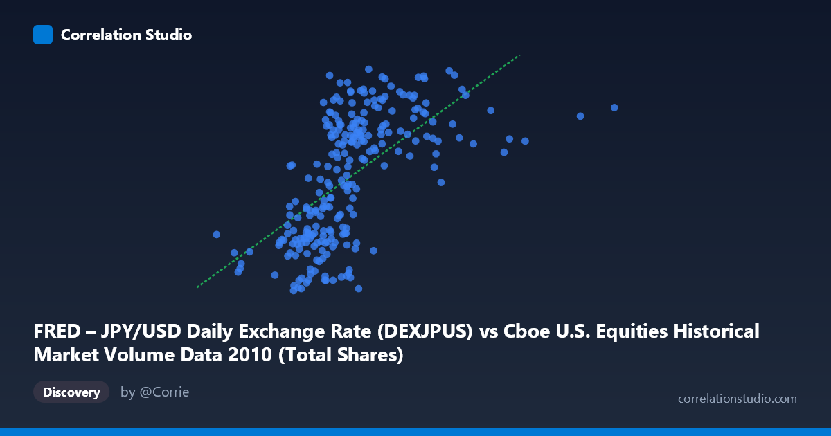
FRED – JPY/USD Daily Exchange Rate (DEXJPUS) vs Cboe U.S. Equities Historical Market Volume Data 2010 (Total Shares)
- Pearson correlation (r)
- 0.6106
- Spearman correlation
- 0.695
- p-value
- 0
- Sample size (n)
- 249
- 95% confidence interval
- 0.5263 to 0.6831
- Granger causality
- None
- Granger optimal lag
- 1
AI analysis
Analysis: JPY/USD Exchange Rate vs. U.S. Equity Market Volume (2010)
Relationship Overview The scatterplot reveals a moderate positive relationship between the FRED JPY/USD daily exchange rate (X-axis, representing daily U.S. equity market volume in notional terms) and total shares traded on Cboe U.S. equities markets (Y-axis). As the X variable increases, Y values tend to rise in a broadly upward pattern, consistent with the positive linear regression slope (y = 1.30383E⁻⁰⁸x + 79.14). However, the scatter is substantial, with considerable vertical spread at nearly all X values, indicating that the linear trend captures only part of the story. The data spans the full 2010 trading year, and the relationship appears to reflect underlying market dynamics rather than a clean mechanical link between these two series.
Correlation Strength and Statistical Significance The Pearson correlation of r = 0.61 indicates a moderate positive association, but the more informative metric is r² = 0.373 — meaning approximately 37.3% of the variance in total shares traded is explained by the X variable. While statistically significant (p ≈ 0, n = 249), this leaves roughly 62.7% of variance unexplained, underscoring that many other forces are at work. The 95% confidence interval [0.53, 0.68] is reasonably tight, suggesting the true population correlation is reliably in the moderate range and not an artifact of sampling. Critically, the Granger causality tests show no significant predictive directionality in either direction (X→Y: F = 0.94, p = 0.33; Y→X: F = 0.82, p = 0.37), meaning neither variable reliably predicts the other temporally with a one-period lag. This is an important caveat: correlation here does not imply any leading-lagging relationship at this resolution.
Patterns, Clusters, and Outliers The sample points reveal several notable structural features. There appears to be a dense central cluster roughly between X = 500M–800M and Y = 83–93, where most trading days concentrate. A smaller but visible upper-right cluster (e.g., points near X = 1.03B, Y = 94.30 and X = 1.16B, Y = 92.03) suggests that high-volume days also tend to see elevated share totals, though the relationship weakens at these extremes. Conversely, lower-left points (e.g., X ≈ 250M, Y = 82.91 and X ≈ 410M, Y = 83.56) show that low-volume days correspond to lower Y values. A few points suggest non-linear behavior — some mid-range X values produce both very high and very low Y readings (e.g., X ≈ 662M produces Y values ranging from 81.3 to 93.2), hinting at heteroscedasticity or regime-dependent behavior within the year.
Confounding Factors and Caveats Several important caveats apply. First, the axis labels appear swapped in the dataset descriptions — the X-axis is labeled as JPY/USD exchange rate data but described as equity volume, and vice versa, which warrants careful verification before drawing conclusions. Second, both series are driven heavily by common macroeconomic and calendar factors in 2010 — post-financial-crisis recovery dynamics, Fed policy, risk-on/risk-off sentiment shifts, and seasonal patterns in equity trading could simultaneously influence both variables, creating spurious or confounded correlation. Third, the single-year scope (2010 only) means findings may not generalize; 2010 was a distinctive year featuring the Flash Crash (May 6) and ongoing European sovereign debt concerns. Finally, the absence of Granger causality at lag-1 does not rule out longer-lag relationships or non-linear temporal dependencies.
Actionable Insights and Further Investigation Given the moderate but unexplained variance and lack of temporal directionality, several follow-up analyses are warranted. Extending the time series beyond 2010 would test whether this correlation is structurally stable or period-specific. Applying non-linear models (e.g., polynomial regression or GAMs) could better capture the heteroscedasticity visible in the mid-range X values. Testing longer Granger causality lags (beyond 1 period) may reveal delayed predictive relationships not captured at lag-1. Additionally, decomposing both series by day-of-week, month, or volatility regime (e.g., pre/post Flash Crash) could isolate whether the correlation is driven by specific market conditions. Finally, controlling for VIX or macro news events would help disentangle genuine co-movement from common factor confounding.
X dataset: Cboe U.S. Equities Historical Market Volume Data 2010
Y dataset: FRED – JPY/USD Daily Exchange Rate
Part of experiment: Daily - Cboe U.S. Equities Historical Market Volume Data 2010 vs FRED – JPY/USD Daily Exchange Rate